MC Techniques Summary for Amplitude Calculation & Phase Space Integration
180 likes | 288 Vues
Learn about matrix element Monte Carlo techniques for amplitude calculation and phase space integration based on Sara Bolognesi's detailed lessons from May 31, 2006. Explore parton shower, hadronization, approximation methods, and numerical integration strategies.

MC Techniques Summary for Amplitude Calculation & Phase Space Integration
E N D
Presentation Transcript
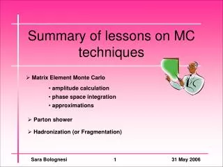
Summary of lessons on MC techniques • Matrix Element Monte Carlo • amplitude calculation • phase space integration • approximations • Parton shower • Hadronization (or Fragmentation) Sara Bolognesi 31 May 2006 1
Parton level simulation Increasing in collider energy Increasing number of final state particles Increasing the complexity of the parton level simulation: More Feynman diagrams and with a complex topology : • increasing of the difficulty in the amplitude calculation • you need to correctly manage the phase space • more efficient integration techniques have to be developed Sara Bolognesi 31 May 2006 2
Amplitude calculation Standard method: TRACE EVALUATION • the number of terms grows with a power 2 of the number of diagrams EX.: with 2 diagrams -> 3 terms • you loose spin info by summing on polarization New technique: HELICITY AMPLITUDE METHODS working with amplitude (not squared!) • smaller cancellations between different terms, the cancellations become more easy to manage so in reality • you keep the spin info: you need to use approximation (ex. m~0) Sara Bolognesi 31 May 2006 3
Spinor formalism Re-write the amplitude as a product of terms each of which represents a “piece” of diagram EXAMPLE: with these pieces you can construct the diagrams for Very simple to computerize the process in an automatic program Sara Bolognesi 31 May 2006 4
Phase space integration • For each intermediate particle you have a propagator so you have a resonance in the amplitude • The dimension of the phase space (i.e. the number of variables on which you have to integrate) grows with 3N-4 (N = number of final particles) You want to have a stable and reliable result and you need it quickly!! • adaptive iterative algorithm • multi-channel technique The main strategy is choose as integration variables those which have the peaks (i.e. align the peaks with the axis) = PHASE SPACE SPLITTING make a change of variable to flat the bumps in the amplitude = IMPORTANCE / STRATIFIED SAMPLING Sara Bolognesi 31 May 2006 5
Phase space splitting Re-write the phase space of N outgoing particles as the product of phase space of N/2 couples of particles where M(j,j+1) are the variables where you expect the bumps in the amplitude EXAMPLE: so you have to choose carefully the splitting accordingly to physics process (eventually you need to use different splitting for the same amplitude -> multi-channel techniques) Sara Bolognesi 31 May 2006 6
Numerical integration We can’t computerize an analytical integration but we can apply a numerical integration (better we know our function -> more efficient and precise could be the integration) MC integration is the best technique: E = estimate of the result N = number of points used to integrate the error on the estimate converges to the real result not very quickly but it’s independent from the integral dimensions (i.e. the number of variables) Techniques to improve the convergence are more than welcome!! • importance sampling • stratified sampling Sara Bolognesi 31 May 2006 7
Importance sampling • THE MAIN IDEA: put more points where the function peaks more • MATHEMATICS: change of variable to pass from x (distributed according with f) to P (rather uniformly distributed) with • PRATICALLY: • choose a probability density function P(x) with those properties • generate uniform random number z • change the variable: • sample f with x Sara Bolognesi 31 May 2006 8
Stratified sampling • THE MAIN IDEA: Put more points where the function varies more quickly • PRATICALLY: Split your integration interval in N different sub-intervals (thanks to the linearity): • put the same amount of points in each intervals • use narrower intervals where the function varies more quickly • MATHEMATICS: The error on the total integral is lower if the error on different sub-intervals is of the same order Sara Bolognesi 31 May 2006 9
Adaptive-iterative algorithm Because you don’t know the shape of the function, you need to learn about that during the integration itself: split the integration domain in sub-intervals where you put the same amount of points at the first iteration points equally distributed on all the domain see where the first integration is less precise at the second iteration put more points here and so on… … but we need to have already the peaks aligned with the axis (thanks to the phase splitting) Sara Bolognesi 31 May 2006 10
Multichannel techniques …but typically you have many peaks in different direction (one peak on the mass of each intermediate resonance) For each channeluse a different mapping i.e. a different set of variables to map your phase space M(bb) ~ MZ M(ev) ~ MW EXAMPLE: M(bev) ~ Mtop M(ev) ~ MW define a probability (ai) of pick up that channel (the best ai are the ones which give roughly the same error for the different channels) Sara Bolognesi 31 May 2006 11
Approximations in M.E. MC MASSLESS APPROXIMATION + to reduce the number ofhelicity configuration that you have to consider - could raise some fictitious singularity -> instability in the MC Anyone MC can’t cover all the phase space NOTE: also without massless approximation the mass of an electron can be a trouble! se e you have to apply clever cuts on the phase space in order to avoid singularities and instability Sara Bolognesi 31 May 2006 12
NARROW WIDTH APPROXIMATION AND PRODUCTION TIMES DECAY In general you can’t consider only a subset of diagrams of your process because • you can loose big interference terms or cancellation effects • you break the Gauge Invariance but you can save the G.I. by forcing your intermediate particles to be on shell = Narrow Width Approximation qq->e+e-e+e- ~ qq->ZZ->e+e-e+e- PRODUCTION TIMES DECAY ~ Mathematically this corresponds to • neglect spin correlation between production and decay of the intermediate particles • approximate the resonance with a Dirac delta - you can’t esteem the acceptance of cuts on the invariant mass - you loose spin info (that affects the angular distributions) and all the irreducible backgrounds + you can use this approx. to introduce NLO corrections Sara Bolognesi 13 31 May 2006
WEIZSECKER-WILLIAM APPROXIMATION The extension of the NWA from s to t channel (i.e. virtual intermediate particle) q2 ~ 0 A sort of PDF = probability to find a photon in an electron scattering of a quasi real photon with a positron EQUIVALENT VECTOR BOSON APPROXIMATION The extension of the WWA from the photon to massive vector boson q2 ~ MV A little more tricky because MV doesn’t belong to the allowed values of q2 (q2<0) scattering of real vector boson A sort of PDF = probability to find a V in a fermion Sara Bolognesi 14 31 May 2006
Parton shower HARD SCATTERING PARTONIC PROCESS HADRONIZATION / FRAGMENTATION high energy (>~100 GeV) “low” energy (~100 MeV) PARTON SHOWER = radiation from initial and final state (ISR/FSR) • bulk of the corrections to the LO process • scale evolution Approximated with only 1->2 split • 1->3 processes i.e. only O(as) considered at each split: • virtual corrections Sara Bolognesi 31 May 2006 15
Bulk of corrections • From a perturbative point of view, we have divergences due to • virtual corrections equal and opposite, they cancel one with the other • soft emission (IR divergences) • collinear emission Multiple emission: ordinate emission from big angles at larger scale to small angles at lower scale: • Physical interpretation: emitted and intermediate particles as partons (constituent) of the initial particle DGLAP equation = probability of splitting, a sort of PDF • MC algorithm • generate a random number 0<r<1 • if r < Prob. of non splitting stop here • else r=Pnosplit(Q2,K2) extract K and simulate splitting (with 4-mom. conservation) Sara Bolognesi 31 May 2006 16
Hadronization Reconstruct the final stable hadrons from partons radiated during the Parton Shower Models to describe the reality (i.e. to fit the data) not a coherent theory (no Lagrangian): PS + hadronization String Fragmentation (Lund model) color exchange (i.e strong force) between quarks represented with a string potential proportional to the quarks distance (string length) when the energy is high, the string crack and give rise to a new couple of quark hadron MC contains an iterative algorithm to reproduce this process with a probabilistic approach Sara Bolognesi 31 May 2006 17
