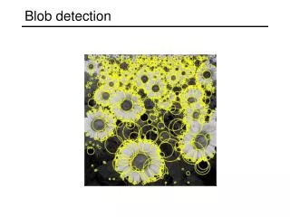
Blob detection
Blob detection. Feature detection with s cale selection. We want to extract features with characteristic scale that is covariant with the image transformation. Blob detection: basic idea.

Blob detection
E N D
Presentation Transcript
Feature detection with scale selection • We want toextract features with characteristic scale that is covariant with the image transformation
Blob detection: basic idea • To detect blobs, convolve the image with a “blob filter” at multiple scales and look for maxima of filter response in the resulting scale space
Blob filter • Laplacian of Gaussian: Circularly symmetric operator for blob detection in 2D
Recall: Edge detection Edge f Derivativeof Gaussian Edge = maximumof derivative Source: S. Seitz
Edge detection, Take 2 Edge f Second derivativeof Gaussian (Laplacian) Edge = zero crossingof second derivative Source: S. Seitz
maximum From edges to blobs • Edge = ripple • Blob = superposition of two ripples Spatial selection: the magnitude of the Laplacianresponse will achieve a maximum at the center ofthe blob, provided the scale of the Laplacian is“matched” to the scale of the blob
original signal(radius=8) increasing σ Scale selection • We want to find the characteristic scale of the blob by convolving it with Laplacians at several scales and looking for the maximum response • However, Laplacian response decays as scale increases:
Scale normalization • The response of a derivative of Gaussian filter to a perfect step edge decreases as σ increases
Scale normalization • The response of a derivative of Gaussian filter to a perfect step edge decreases as σ increases • To keep response the same (scale-invariant), must multiply Gaussian derivative by σ • Laplacian is the second Gaussian derivative, so it must be multiplied by σ2
Scale-normalized Laplacian response maximum Effect of scale normalization Original signal Unnormalized Laplacian response
Blob detection in 2D • Laplacian of Gaussian: Circularly symmetric operator for blob detection in 2D Scale-normalized:
Scale selection • At what scale does the Laplacian achieve a maximum response to a binary circle of radius r? r image Laplacian
Scale selection • At what scale does the Laplacian achieve a maximum response to a binary circle of radius r? • To get maximum response, the zeros of the Laplacian have to be aligned with the circle • The Laplacian is given by (up to scale): • Therefore, the maximum response occurs at circle r 0 Laplacian image
Characteristic scale • We define the characteristic scale of a blob as the scale that produces peak of Laplacian response in the blob center characteristic scale T. Lindeberg (1998). "Feature detection with automatic scale selection."International Journal of Computer Vision30 (2): pp 77--116.
Scale-space blob detector • Convolve image with scale-normalized Laplacian at several scales
Scale-space blob detector • Convolve image with scale-normalized Laplacian at several scales • Find maxima of squared Laplacian response in scale-space
Efficient implementation • Approximating the Laplacian with a difference of Gaussians: (Laplacian) (Difference of Gaussians)
Efficient implementation David G. Lowe. "Distinctive image features from scale-invariant keypoints.”IJCV 60 (2), pp. 91-110, 2004.
From feature detection to feature description • Scaled and rotated versions of the same neighborhood will give rise to blobs that are related by the same transformation • What to do if we want to compare the appearance of these image regions? • Normalization: transform these regions into same-size circles • Problem: rotational ambiguity
p 2 0 Eliminating rotation ambiguity • To assign a unique orientation to circular image windows: • Create histogram of local gradient directions in the patch • Assign canonical orientation at peak of smoothed histogram
SIFT features • Detected features with characteristic scales and orientations: David G. Lowe. "Distinctive image features from scale-invariant keypoints.”IJCV 60 (2), pp. 91-110, 2004.
SIFT descriptors David G. Lowe. "Distinctive image features from scale-invariant keypoints.”IJCV 60 (2), pp. 91-110, 2004.
Invariance vs. covariance • Invariance: • features(transform(image)) = features(image) • Covariance: • features(transform(image)) = transform(features(image)) Covariant detection => invariant description
Affine adaptation • Affine transformation approximates viewpoint changes for roughly planar objects and roughly orthographic cameras
direction of the fastest change direction of the slowest change (max)-1/2 (min)-1/2 Affine adaptation Consider the second moment matrix of the window containing the blob: Recall: This ellipse visualizes the “characteristic shape” of the window
Affine adaptation example Scale-invariant regions (blobs)
Affine adaptation example Affine-adapted blobs