GEO7600 Inverse Theory 09 Oct 2008

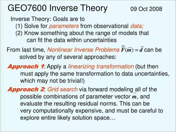
1. GEO7600 Inverse Theory 09 Oct 2008 Inverse Theory: Goals are to (1) Solve for parameters from observational data; (2) Know something about the range of models that can fit the data within uncertainties From last time, Nonlinear Inverse ProblemsF(m) = d can be solved by any of several approaches: Approach 1: Apply a linearizing transformation (but then must apply the same transformation to data uncertainties, which may not be trivial!) Approach 2: Grid search via forward modeling all of the possible combinations of parameter vector m, and evaluate the resulting residual norms. This can be very computationally expensive, and must be careful to explore entire likely solution space…

2. Inverse Theory for Nonlinear Problems Approach 3: Iterative solution based on gradient search: Multi-dimensional Taylor Series expansion about some initial model “guess” m0 is given by: where We want to find the m that approximates the difference between m0 & mtrue. For N data points, with sensitivity coefficients

3. To get the desired m, we seek the m that satisfies: Substituting for in the Taylor Series approximation, We can solve for m using the same linear pseudo-inverse techniques we have used up to now! Because we truncated the Taylor Series at first order, our estimate is only accurate to … But we can update our model “guess” to be and then iterate…

4. Since each new model mk should be closer to mtrue than the previous, and the error in each successive estimate decreases proportional to the length-squared of m, the model estimate should converge to mtrue(subject to errors in d as in the linear case). The sensitivity coefficients are determined for i = 1,2,…,N data and j = 1,2,…,M model parameters so G is an NxM matrix. Note however that this implies the physical model must be differentiable… Consider as example fitting an exponential: Will have: &

5. Note that most of the same tools we used for the linear problem (e.g., estimates of parameter error from the parameter covariance matrix; model resolution and covariance matrices;  parameter etc.) still apply to the iterative solution for a nonlinear model… The main difference being that we apply these metrics to the final (iterated) model estimate using the sensitivity matrix G of the best-fitting model.