Download
1 / 18
180 likes | 328 Vues
This presentation by Vikram Gupta discusses the complex nature of spatial localization through the integration of visual and auditory signals. It reviews how inconsistent spatial cues can affect our sensory perception, emphasizing a Bayesian framework that blends information from different sensory modalities. The talk details methods like Maximum Likelihood Estimation (MLE) and explores conditions under which these integrations occur, supported by empirical data from experiments. The findings reveal how priors and variances influence sensory integration, providing insights into the biological basis of these processes.

E N D
Authors: Peter W. Battaglia, Robert A. Jacobs, and Richard N. Aslin Bayesian integration of visual and auditory signals for spatial localization COGS 272, Spring 2010 Instructor: Prof. Angela Yu Presenter: Vikram Gupta
Outline • Introduction • Background • Methods • Procedure • Results • Discussion
IntroductionSpatial Localization is Complex • Integration of multiple sensory and motor signals • Sensory: binaural time, phase, intensity difference • Motor: orientation of the head
Introduction∫ Inconsistent Spatial Cues • Typically, we receive consistent spatial cues • What if this is not true? • Ex: Movie theater, television • Visual capture • Vision dominates over conflicting auditory cue. • Ex: recalibration in juvenile owl • Optimal?
BackgroundModels for inconsistent cue integration • Winner Take All (ex. vision capture) • Dominant signal exclusively decides • Blend information from sensory sources • Is blending statistically optimal? • Example: Maximum Likelihood Estimate • Assumption independent sensory signals, normal dist.
BackgroundMLE Example Impact of reliability on MLE estimate
MLE Model • Is Normal distribution a good estimate of neural coding of sensory input? • Does this integration always occur? Or are there qualifying conditions? • Does it make sense to integrate if • Lv* and La* are far apart? • v and a are temporally separated?
Schematic of MLE Integration • Ernst, 2006 (MLE integration for haptic and visual input
Experiment • Vision capture or MLE match empirical data? • Method summary: • Noise is produced at 1 of 7 locations 1.50 apart • Visual stimulus has noise at 5 levels • 10%, 23%, 36%, 49%, 62% • Single sensory modality trial (Audio / noisy Visual ) MLE parameters predict performance for Audio + noisy Visual compare with Empirical data
Experiment S C • Single-modality • Standard stimuli followed by comparison • Is C Left / Right of S? • Bimodal • Standard stimuli has Audio and Visual apart from center • Audio and visual Comparison stimuli are co-located. • Only 1 subject aware of spatial discrepancy in S
Results (1 subject) • Cumulative normal distribution fits to data • Mean and variance are used for MLE model • Wv receives high value when visual noise is low • Wa receives high value when visual noise is high
Results (MLE Estimate of sensory input) • rt = 1 comparison to the right of standard • pt = , probability of rt, given mean and variance • R = set of responses to the independent trials • Assuming normal distribution, MLE estimate of mean and variance parameters • µml = 1/T * (∑ rt) σ2ml = 1/T * (rt - µml) 2
L* based on MLE estimates • Mean is calculated according to above weighted average • Variance is smaller than either P(L|v) or P(L|a)
L* based on MLE estimates • MLE estimate for wv and wa are found by maximizing RHS of (3) and using (6) • tau is scale parameter or slope
Results (bi-modal, same subject, all subjects) • Standard stimulus • Visual -1.50 • Audio 1.50 • Point of Subjective Equality • -1.10 for low visual noise • 0.10 for high noise • Visual input dominates at low noise • Equal weight at high noise
Empirical vs. MLE • MLE estimates for visual weight are significantly lower than the empirical results. • A Bayesian model with a prior that reduces variance in visual-only trials provides a good regression fit for the data.
Bayesian (MAP) Cue Integration • For visual only trials, instead of using MLE for mean and variance, we multiply the RHS above with the probability of the occurrence of the normal distribution • mean is assumed to have a uniform distribution. • variance is assumed to have inverse gamma distribution with parameters biased for small variance.
Discussion • Bayesian approach is a hybrid of MLE and visual capture models. • How are variances encoded? • How are priors encoded? • How does temporal separation in cues impact sensory integration? • Biological basis for Bayesian cue integration?