Data types
Data types. Outline Primitive data types Structured data types Strings Enumerated types Arrays Records Pointers. Reading assignment. Arrays. An array represents a mapping: index_type component_type

Data types
E N D
Presentation Transcript
Data types Outline • Primitive data types • Structured data types • Strings • Enumerated types • Arrays • Records • Pointers Reading assignment
Arrays An array represents a mapping: index_type component_type The index type must be a discrete type (integer, character, enumeration etc). In some languages this type is specified implicitly: an array of size N is indexed 0…N-1 in C++ / Java / Perl, but in Fortran it is 1…N. In Algol, Pascal, Ada the lower and upper bound must be both given. There are normally few restrictions on the component type (in some languages we can even have arrays of procedures or files).
Multidimensional arrays Multidimensional arrays can be defined in two ways (for simplicity, we show only dimension 2): index_type1 index_type2 component_type This corresponds to references such as A[I,J]. Algol, Pascal, Ada work like this. index_type1 (index_type2 component_type) This corresponds to references such as A[I][J]. Java works like this. Perl sticks to one dimension
Operations on arrays (1) select an element (get or change its value): A[J] select a slice of an array: (read the textbook, Section 6.5.7) assign a complete array to a complete array: A := B; There is an implicit loop here.
Operations on arrays (2) Compute an expression with complete arrays (this is possible in extendible or specialized languages, for example in Ada): V := W + U; If V, W, U are arrays, this may denote array addition. All three arrays must be compatible (the same index and component type), and addition is probably carried out element by element.
Subscript binding static: fixed size, static allocation this is done in older Fortran. semistatic: fixed size, dynamic allocation Pascal. semidynamic: size determined at run time, dynamic allocation Ada dynamic: size fluctuates during execution, flexible allocation required Algol 68, APL—both little used...
Array-type constants and initialization Many languages allow initialization of arrays to be specified together with declarations: C int vector [] = {10,20,30}; Ada vector: array(0..2) of integer := (10,20,30); Array constants in Ada temp is array(mo..su)of -40..40; T: temp; T := (15,12,18,22,22,30,22); T := (mo=>15, we=>18, tu=>12, sa=>30, others=>22); T := (15,12,18, sa=>30, others=>22);
Implementing arrays (1) The only issue is how to store arrays and access their elements—operations on the component type decide how the elements are manipulated. An array is represented during execution by an array descriptor. It tells us about: the index type, the component type, the address of the array, that is, the data.
Implementing arrays (2) Specifically, we need: the lower and upper bound (for subscript checking), the base address of the array, the size of an element. We also need the subscript—it gives us the offset (from the base) in the memory area allocated to the array. A multi-dimensional array will be represented by a descriptor with more lower-upper bound pairs.
Implementing multidimensional arrays Row major order (second subscript increases faster) Column major order (first subscript increases faster)
Implementing multidimensional arrays (2) Suppose that we have this array: A: array [LOW1..HIGH1, LOW2..HIGH2] of ELT; where the size of each entity of type ELT is SIZE. This calculation is done for row-major (calculations for column-major are quite similar). We need the base—for example, the address LOC of A[LOW1, LOW2].
Implementing multidimensional arrays (3) We can calculate the address of A[I,J] in the row-major order, given the base. Let the length of each row in the array be: ROWLENGTH = HIGH2 - LOW2 + 1 The address of A[I,J] is: (I - LOW1) * ROWLENGTH * SIZE + (J - LOW2) * SIZE + LOC
Implementing multidimensional arrays (4) Here is an example. VEC: array [1..10, 5..24] of integer; The length of each row in the array is: ROWLENGTH = 24 - 5 + 1 = 20 Let the base address be 1000, and let the size of an integer be 4. The address of VEC[i,j] is: (i - 1) * 20 * 4 + (j - 5) * 4 + 1000 For example, VEC[7,16] is located in 4 bytes at 1524 = (7 - 1) * 20 * 4 + (16 - 5) * 4 + 1000
Languages without arrays A final word on arrays: they are not supported by standard Prolog and pure Scheme. An array can be simulated by a list, which is the basic data structure in Scheme and a very important data structure in Prolog. Assume that the index type is always 1..N. Treat a list of N elements: [x1, x2, ..., xN] (Prolog) (x1 x2 ... xN) (Scheme) as the (structured) value of an array
Back to pointers [Note: We’re skipping 6.9.9] A pointer variable has addresses as values (and a special address nil or null for "no value"). They are used primarily to build structures with unpredictable shapes and sizes—lists, trees, graphs—from small fragments allocated dynamically at run time. A pointer to a procedure is possible, but normally we have pointers to data (simple and composite). An address, a value and usually a type of a data item together make up a variable. We call it an anonymous variable: no name is bound to it. Its value is accessed by dereferencing the pointer.
p 17 Back to pointers (2) Pointers in Pascal are quite well designed. Note that, as with normal named variables, in this: p^ := 23; we mean the address of p^ (the value of p). In this: m := p^; we mean the value of p^. value(p) = value(p^) = 17
Pointer variable creation A pointer variable is declared explicitly and has the scope and lifetime as usual. An anonymous variable has no scope (because it has no name) and its lifetime is determined by the programmer. It is created (in a special memory area called heap) by the programmer, for example: new(p); in Pascal p = malloc(4); in C and destroyed by the programmer: dispose(p); in Pascal free(p); in C
Pointer variable creation (2) If an anonymous variable exists outside the scope of the explicit pointer variable, we have "garbage" (a lost object). If an anonymous variable has been destroyed inside the scope of the explicit pointer variable, we have a dangling reference. new(p); p^ := 23; dispose(p); ...... if p^ > 0 {???}
Pointer variable creation (2) Producing garbage, an example in Pascal: new(p); p^ := 23; new(p); {the anonymous variable with the value 23 becomes inaccessible} Garbage collection is the process of reclaiming inaccessible storage. It is usually complex and costly. It is essential in languages whose implementation relies on pointers: Lisp, Prolog.
Pointers: types and operators Pointers in PL/I are typeless. In Pascal, Ada, C they are declared as pointers to types, so that a dereferenced pointer (p^, *p) has a fixed type. Operations on pointers in C are quite rich: char b, c; c = '\007'; b = *((&c - 1) + 1); putchar(b);