Supply-Chain Design
Supply-Chain Design. Chapter 9. Input flow of materials. Inventory level. Scrap flow. Output flow of materials. Creation of Inventory. Figure 9.3. Work in process. Raw materials. Finished goods. Supplier Manufacturing plant Distribution center Retailer.

Supply-Chain Design
E N D
Presentation Transcript
Supply-Chain Design Chapter 9
Input flow of materials Inventory level Scrap flow Output flow of materials Creation of Inventory Figure 9.3
Work in process Raw materials Finished goods Supplier Manufacturing plant Distribution center Retailer Inventory at Different Stocking Points Figure 9.4
Customer Customer Customer Customer Distribution center Distribution center Manufacturer Tier 1 Tier 2 Tier 3 Legend Supplier of services Supplier of materials Supply Chain Figure 9.5
9,000 – 7,000 – 5,000 – 3,000 – 0 – Package supplier’s weekly orders to cardboard supplier Manufacturer’s weekly orders to package supplier Retailers’ daily orders to manufacturer Consumers’ daily demand Order Quantity Time Supply Chain Dynamics for Facial Tissue Figure 9.6
Supermarket A distribution center Supermarket B distribution center Distribution domain of responsibility Transportation services supplier FG storage Transformation process and WIP storage Production domain of responsibility Purchasing domain of responsibility RM storage Egg supplier Sugar supplier Flour supplier Chocolate chips supplier Maintenance services supplier Materials Management Figure 9.7
$2 million ($10 million)/(52 weeks) Weeks of supply = = 10.4 weeks $10 million $2 million Inventory turns = = 5 turns/year Inventory Measures Average inventory = $2 million Cost of goods sold = $10 million 52 business weeks per year Example 9.1
TABLE 9.1 SUPPLY–CHAIN PROCESS MEASURES Customer Relationship Order Fulfillment Supplier Relationship • Percent of orders taken accurately • Time to complete the order placement process • Customer satisfaction with the order placement process • Percent of incomplete orders shipped • Percent of orders shipped on time • Time to fulfill the order • Percent of botched services or returned items • Cost to produce the service or item • Customer satisfaction with the order fulfillment process • Percent of suppliers’ deliveries on time • Suppliers’ lead times • Percent defects in services and purchased materials • Cost of services and purchased materials Supply-Chain Process Measures
TABLE 9.2 ENVIRONMENTS BEST SUITED FOR EFFICIENT AND RESPONSIVE SUPPLY CHAINS Supply-Chain Environments FactorEfficient Supply ChainsResponsive Supply Chains Demand Predictable, low Unpredictable, high forecast errors forecast errors Competitive Low cost, consistent Development speed, fast priorities quality, on-time delivery times, delivery customization, volume flexibility, variety, top quality New-service/ Infrequent Frequent product introduction Contribution Low High margins Product variety Low High
TABLE 9.3 DESIGN FEATURES FOR EFFICIENT AND RESPONSIVE SUPPLY CHAINS Supply-Chain Design FactorEfficient Supply ChainsResponsive Supply Chains Operation Make-to-stock or Assemble-to-order, make- strategy standardized services; to-order, or customized emphasize high services; emphasize volume, standardized service or product services or products variety Capacity Low High cushion Inventory Low, enable high As needed to enable fast investment inventory turns delivery time Lead time Shorten, but do not Shorten aggressively increase costs Supplier Emphasize low prices, Emphasize fast delivery selection consistent quality, on- time, customization, time delivery variety, volume flexibility, top quality
Location Chapter 10
Reasons for Globalization • Improved transportation and communication technologies • Loosened regulations on financial institutions • Increased demand for imported services and goods • Reduced import quotas and other international trade barriers
Managing Global Operations • Other Languages • Different Norms and Customs • Workforce Management • Unfamiliar Laws and Regulations • Unexpected Cost Mix
Location Decisions - Manufacturing • Favorable Labor Climate • Proximity to Markets • Quality of Life • Proximity to Suppliers • Proximity to Parent Company • Utilities, Taxes, and Real Estate Costs
Location Decisions - Services • Proximity to Customers • Transportation Costs and Proximity to Markets • Location of Competitors • Site-Specific Factors
North Erie Scranton State College Pittsburgh Harrisburg Philadelphia Uniontown Location Health-Watch Example 10.1
Erie Scranton State College Pittsburgh Harrisburg Philadelphia Uniontown Location Health-Watch North Location Factor Weight Score Total patient miles per month 25 4 Facility utilization 20 3 Average time per emergency trip 20 3 Expressway accessibility 15 4 Land and construction costs 10 1 Employee preference 10 5 Example 10.1
Erie Scranton State College Pittsburgh Harrisburg Philadelphia Uniontown Location Health-Watch North Weighted Score Location Factor Weight Score Total patient miles per month 25 4 Facility utilization 20 3 Average time per emergency trip 20 3 Expressway accessibility 15 4 Land and construction costs 10 1 Employee preference 10 5 WS = (25 x 4) Example 10.1
Erie Scranton State College Pittsburgh Harrisburg Philadelphia Uniontown Location Health-Watch North Weighted Score Location Factor Weight Score Total patient miles per month 25 4 Facility utilization 20 3 Average time per emergency trip 20 3 Expressway accessibility 15 4 Land and construction costs 10 1 Employee preference 10 5 WS = (25 x 4) + (20 x 3) + (20 x 3) + (15 x 4) + (10 x 1) + (10 x 5) Example 10.1
Erie Scranton State College Pittsburgh Harrisburg Philadelphia Uniontown Location Health-Watch North Weighted Score Location Factor Weight Score Total patient miles per month 25 4 Facility utilization 20 3 Average time per emergency trip 20 3 Expressway accessibility 15 4 Land and construction costs 10 1 Employee preference 10 5 WS = 340 Example 10.1
453.5 68 205.5 68 x* = y* = Census Population Tract (x, y) (l) lxly A (2.5, 4.5) 2 5 9 B (2.5, 2.5) 5 12.5 12.5 C (5.5, 4.5) 10 55 45 D (5, 2) 7 35 14 E (8, 5) 10 80 50 F (7, 2) 20 140 40 G (9, 2.5) 14 126 35 Totals 68 453.5 205.5 LocationCenter of Gravity Approach Example 10.2
x* = 6.67 y* = 3.02 Census Population Tract (x, y) (l) lxly A (2.5, 4.5) 2 5 9 B (2.5, 2.5) 5 12.5 12.5 C (5.5, 4.5) 10 55 45 D (5, 2) 7 35 14 E (8, 5) 10 80 50 F (7, 2) 20 140 40 G (9, 2.5) 14 126 35 Totals 68 453.5 205.5 LocationCenter of Gravity Approach Example 10.2
Location Break-Even Analysis for 20,000 units Fixed Costs Variable Costs Total Costs Community per Year per Unit (Fixed + Variable) A $150,000 $62 B $300,000 $38 C $500,000 $24 D $600,000 $30 Total Variable Costs $62 (20,000) Example 10.3
Location Break-Even Analysis for 20,000 units Fixed Costs Variable Costs Total Costs Community per Year per Unit (Fixed + Variable) A $150,000 $62 B $300,000 $38 C $500,000 $24 D $600,000 $30 Total Variable Costs $62 (20,000) = $1,240,000 Example 10.3
Location Break-Even Analysis for 20,000 units Fixed Costs Variable Costs Total Costs Community per Year per Unit (Fixed + Variable) A $150,000 $62 $1,390,000 B $300,000 $38 C $500,000 $24 D $600,000 $30 Total Variable Costs $62 (20,000) = $1,240,000 Example 10.3
Location Break-Even Analysis for 20,000 units Fixed Costs Variable Costs Total Costs Community per Year per Unit (Fixed + Variable) A $150,000 $62 $1,390,000 B $300,000 $38 C $500,000 $24 D $600,000 $30 Total Variable Costs $62 (20,000) = $1,240,000 Example 10.3
Location Break-Even Analysis for 20,000 units Fixed Costs Variable Costs Total Costs Community per Year per Unit (Fixed + Variable) A $150,000 $62 $1,390,000 B $300,000 $38 $1,060,000 C $500,000 $24 $ 980,000 D $600,000 $30 $1,200,000 Example 10.3
Fixed Costs Total Costs Community per Year (Fixed + Variable) A $150,000 $1,390,000 B $300,000 $1,060,000 C $500,000 $ 980,000 D $600,000 $1,200,000 1600 A (20, 1390) 1400 (20, 1200) D 1200 B (20, 1060) C 1000 Annual cost (thousands of dollars) (20, 980) 800 Break-even point 600 Break-even point 400 200 A best B best C best 0 2 4 6 8 10 12 14 16 18 20 22 6.25 14.3 Q (thousands of units) Location Break-Even Analysis Example 10.3
Lean Systems Chapter 11
Characteristics of Lean Systems • Pull method of materials flow • Consistent quality • Small lot sizes • Uniform workstation loads • Standardized components and work methods • Close supplier ties • Flexible workforce • Line flows • Automation • Preventive maintenance
Unreliable suppliers Capacity imbalance Scrap Continuous Improvement with Lean Systems Figure 11.1
Single-Card Kanban System • Each container must have a card • Assembly always withdraws from fabrication (pull system) • Containers cannot be moved without a kanban • Containers should contain the same number of parts • Only good parts are passed along • Production should not exceed authorization Part Number: 1234567Z Location: Aisle 5 Bin 47 Lot Quantity: 6 Supplier: WS 83 Customer: WS 116 KANBAN
d( w + p )( 1 + a ) c k = d = 2000 units/day p = 0.02 day a = 0.10 w = 0.08 day c = 22 units Number of Containers Westerville Auto Parts Example 11.1
d = 2000 units/day p = 0.02 day a = 0.10 w = 0.08 day c = 22 units Number of Containers Westerville Auto Parts 2000( 0.08 + 0.02 )( 1 + 0.10 ) 22 k = Example 11.1
d = 2000 units/day p = 0.02 day a = 0.10 w = 0.08 day c = 22 units Number of Containers Westerville Auto Parts k = 10 containers Example 11.1
Operational Benefits • Reduce space requirements • Reduce inventory investment • Reduce lead times • Increase labor productivity • Increase equipment utilization • Reduce paperwork and simplify planning systems • Valid priorities for scheduling • Workforce participation • Increase service/product quality