Download
1 / 16
160 likes | 297 Vues
Special Topics in Geo-Business Data Analysis. Week 3 Covering Topic 6 Spatial Interpolation. Roving Window (count). Point Density analysis identifies the number of customers with a specified distance of each grid location. Point Density Analysis. (Berry).

E N D
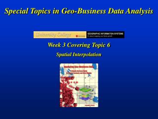
Special Topics in Geo-Business Data Analysis Week 3 Covering Topic 6 Spatial Interpolation
Roving Window (count) Point Density analysis identifies the number of customers with a specified distance of each grid location Point Density Analysis (Berry)
Pockets of unusually high customer density are identified as more than one standard deviation above the mean Identifying Unusually High Density (Berry)
Identifying Customer Territories Clustering on the latitude and longitude coordinates of point locations identify customer territories (Berry)
Mapped data are characterized by their geographic distribution (maps on the left) and their numeric distribution (descriptive statistics and histogram on the right) Map View vs. Data View Geographic Distribution Numeric Distribution (Berry)
The spatial distribution implied by a set of discrete sample points can be estimated by iterative smoothing of the point values Estimating the Geographic Distribution (Berry)
A variogram plot depicts the relationship between distance and measurement similarity (spatial autocorrelation) Spatial Autocorrelation (Variogram) “…nearby things are more alike than distant things” (Berry)
Spatial interpolation involves fitting a continuous surface to sample points Spatial Interpolation Mechanics Roving Window (average) (Berry)
Inverse distance weighted interpolation weight-averages sample values within a roving window Inverse Distance Weighted Technique (Berry)
1 2 3 4 5 6 7 8 9 10 11 12 13 14 15 16 X X Example Calculations for Inverse Distance Squared Interpolation Example Calculations (IDW) 11 16 15 14 (Berry)
Title A wizard interface guides a user through the necessary steps for interpolating sample data MapCalc Spatial Interpolation Wizard (Berry)
Spatial comparison of the project area average and the IDW interpolated surface Comparing Geographic Distributions (IDW vs. Avg) (Berry)
Comparison Statistics (IDW vs. Avg) Statistics summarizing the difference between the IDW surface and the Average …big difference— more than 75 % of the project area is more than +/- 10 units different (Berry)
Comparing Geographic Distributions (IDW vs Krig) Spatial comparison of IDW and Krig interpolated surfaces (Berry)
A residual analysis table identifies the relative performance of average, IDW and Krig estimates Evaluating Interpolation Performance (Berry)
Spatial dependency in continuously mapped data involves summarizing the data values within a “roving window” that is moved throughout a map Mapping Spatial Dependency …compares the difference in values between the adjacent neighbors (doughnut hole) and distant neighbors (doughnut), assigns the spatial dependency index to the center cell location then moves to next location (Berry)