Virtual Data Management for Grid Computing
Virtual Data Management for Grid Computing. Michael Wilde Argonne National Laboratory wilde@mcs.anl.gov Gaurang Mehta, Karan Vahi Center for Grid Technologies USC Information Sciences Institute gmehta,vahi @isi.edu. Outline. The concept of Virtual Data

Virtual Data Management for Grid Computing
E N D
Presentation Transcript
Virtual Data Management for Grid Computing Michael Wilde Argonne National Laboratory wilde@mcs.anl.gov Gaurang Mehta, Karan Vahi Center for Grid Technologies USC Information Sciences Institute gmehta,vahi @isi.edu
Outline • The concept of Virtual Data • The Virtual Data System and Language • Tools and approach for Running on the Grid • Pegasus: Grid Workflow Planning • Virtual Data Applications on the Grid • Research issues
The Virtual Data Concept Enhance scientific productivity through: • Discovery and application of datasets and programs at petabyte scale • Enabling use of a worldwide data grid as a scientific workstation Virtual Data enables this approach by creating datasets from workflow “recipes” and recording their provenance.
Virtual Data Concept • Motivated by next generation data-intensive applications • Enormous quantities of data, petabyte-scale • The need to discover, access, explore, and analyze diverse distributed data sources • The need to organize, archive, schedule, and explain scientific workflows • The need to share data products and the resources needed to produce and store them
GriPhyN – The Grid Physics Network • NSF-funded IT research project • Supports the concept of Virtual Data, where data is materialized on demand • Data can exist on some data resource and be directly accessible • Data can exist only in a form of a recipe • The GriPhyN Virtual Data System can seamlessly deliver the data to the user or application regardless of the form in which the data exists • GriPhyN targets applications in high-energy physics, gravitational-wave physics and astronomy
Virtual Data System Capabilities Producing data from transformations with uniform, precise data interface descriptions enables… • Discovery: finding and understanding datasets and transformations • Workflow: structured paradigm for organizing, locating, specifying, & producing scientific datasets • Forming new workflow • Building new workflow from existing patterns • Managing change • Planning: automated to make the Grid transparent • Audit: explanation and validation via provenance
Virtual Data Example:Galaxy Cluster Search DAG Sloan Data Galaxy cluster size distribution Jim Annis, Steve Kent, Vijay Sehkri, Fermilab, Michael Milligan, Yong Zhao, University of Chicago
mass = 200 decay = bb mass = 200 mass = 200 decay = ZZ mass = 200 decay = WW stability = 3 mass = 200 decay = WW mass = 200 decay = WW stability = 1 mass = 200 event = 8 mass = 200 decay = WW stability = 1 event = 8 mass = 200 plot = 1 mass = 200 decay = WW event = 8 mass = 200 decay = WW stability = 1 plot = 1 mass = 200 decay = WW plot = 1 Virtual Data Application: High Energy Physics Data Analysis mass = 200 decay = WW stability = 1 LowPt = 20 HighPt = 10000 Work and slide by Rick Cavanaugh and Dimitri Bourilkov, University of Florida
Lifecycle of Virtual Data I have some subject images, what analyses are available? which can be applied to this format? I need to document the devices and methods used to measure the data, and keep track of the analysis steps applied to the data. I’ve come across some interesting data, but I need to understand the nature of the analyses applied when it was constructed before I can trust it for my purposes. I want to apply an image registration program to thousands of objects. If the results already exist, I’ll save weeks of computation.
psearch –t 10 … file1 file8 simulate –t 10 … file1 file1 File3,4,5 file2 reformat –f fz … file7 conv –I esd –o aod summarize –t 10 … file6 Virtual Data Scenario Manage workflow; Update workflow following changes On-demand data generation Explain provenance, e.g. for file8: • psearch –t 10 –i file3 file4 file5 –o file8summarize –t 10 –i file6 –o file7reformat –f fz –i file2 –o file3 file4 file5 conv –l esd –o aod –i file 2 –o file6simulate –t 10 –o file1 file2
Abstract Workflow VDL and Abstract Workflow VDL descriptions User request data file “c”
Example Workflow Reduction • Original abstract workflow • If “b” already exists (as determined by query to the RLS), the workflow can be reduced
Mapping from abstract to concrete • Query RLS, MDS, and TC, schedule computation and data movement
Workflow management in GriPhyN • Workflow Generation: how do you describe the workflow (at various levels of abstraction)? (Virtual Data Language and catalog “VDC”)) • Workflow Mapping/Refinement: how do you map an abstract workflow representation to an executable form? (“Planners”: Pegasus) • Workflow Execution: how to you reliably execute the workflow? (Condor’s DAGMan)
Executable Workflow Construction • VDL tools used to build an abstract workflow based on VDL descriptions • Planners (e.g. Pegasus) take the abstract workflow and produce an executable workflow for the Grid or other environments • Workflow executors (“enactment engines”) like Condor DAGMan execute the workflow
Terms • Abstract Workflow (DAX) • Expressed in terms of logical entities • Specifies all logical files required to generate the desired data product from scratch • Dependencies between the jobs • Analogous to build style dag • Concrete Workflow • Expressed in terms of physical entities • Specifies the location of the data and executables • Analogous to a make style dag
Outline • The concept of Virtual Data • The Virtual Data System and Language • Tools and Approach for Running on the Grid • Pegasus: Grid Workflow Planning • Virtual Data Applications on the Grid • Research issues
VDL: Virtual Data LanguageDescribes Data Transformations • Transformation - “TR” • Abstract template of program invocation • Similar to "function definition" • Derivation – “DV” • “Function call” to a Transformation • Store past and future: • A record of how data products were generated • A recipe of how data products can be generated • Invocation • Record of a Derivation execution
Example Transformation TR t1( out a2, in a1, none pa = "500", none env = "100000" ) { argument = "-p "${pa}; argument = "-f "${a1}; argument = "-x –y"; argument stdout = ${a2}; profile env.MAXMEM = ${env}; } $a1 t1 $a2
Example Derivations DV d1->t1 (env="20000", pa="600",a2=@{out:run1.exp15.T1932.summary},a1=@{in:run1.exp15.T1932.raw}, ); DV d2->t1 (a1=@{in:run1.exp16.T1918.raw},a2=@{out.run1.exp16.T1918.summary} );
Workflow from File Dependencies file1 TR tr1(in a1, out a2) { argument stdin = ${a1}; argument stdout = ${a2}; } TR tr2(in a1, out a2) { argument stdin = ${a1}; argument stdout = ${a2}; } DV x1->tr1(a1=@{in:file1}, a2=@{out:file2}); DV x2->tr2(a1=@{in:file2}, a2=@{out:file3}); x1 file2 x2 file3
Example Workflow • Complex structure • Fan-in • Fan-out • "left" and "right" can run in parallel • Uses input file • Register with RLS • Complex file dependencies • Glues workflow preprocess findrange findrange analyze
Workflow step "preprocess" • TR preprocess turns f.a into f.b1 and f.b2 TR preprocess( output b[], input a ) {argument = "-a top";argument = " –i "${input:a};argument = " –o " ${output:b}; } • Makes use of the "list" feature of VDL • Generates 0..N output files. • Number file files depend on the caller.
Workflow step "findrange" • Turns two inputs into one output TR findrange( output b, input a1, input a2,none name="findrange", none p="0.0" ) {argument = "-a "${name};argument = " –i " ${a1} " " ${a2};argument = " –o " ${b};argument = " –p " ${p}; } • Uses the default argument feature
Can also use list[] parameters TR findrange( output b, input a[],none name="findrange", none p="0.0" ) {argument = "-a "${name};argument = " –i " ${" "|a};argument = " –o " ${b};argument = " –p " ${p}; }
Workflow step "analyze" • Combines intermediary results TR analyze( output b, input a[] ) {argument = "-a bottom";argument = " –i " ${a};argument = " –o " ${b}; }
Complete VDL workflow • Generate appropriate derivations DV top->preprocess( b=[ @{out:"f.b1"}, @{ out:"f.b2"} ], a=@{in:"f.a"} ); DV left->findrange( b=@{out:"f.c1"}, a2=@{in:"f.b2"}, a1=@{in:"f.b1"}, name="left", p="0.5" ); DV right->findrange( b=@{out:"f.c2"}, a2=@{in:"f.b2"}, a1=@{in:"f.b1"}, name="right" ); DV bottom->analyze( b=@{out:"f.d"}, a=[ @{in:"f.c1"}, @{in:"f.c2"} );
Compound Transformations • Using compound TR • Permits composition of complex TRs from basic ones • Calls are independent • unless linked through LFN • A Call is effectively an anonymous derivation • Late instantiation at workflow generation time • Permits bundling of repetitive workflows • Model: Function calls nested within a function definition
Compound Transformations (cont) • TR diamond bundles black-diamonds TR diamond( out fd, io fc1, io fc2, io fb1, io fb2, in fa, p1, p2 ) { call preprocess( a=${fa}, b=[ ${out:fb1}, ${out:fb2} ] ); call findrange( a1=${in:fb1}, a2=${in:fb2}, name="LEFT", p=${p1}, b=${out:fc1} ); call findrange( a1=${in:fb1}, a2=${in:fb2}, name="RIGHT", p=${p2}, b=${out:fc2} ); call analyze( a=[ ${in:fc1}, ${in:fc2} ], b=${fd} ); }
Compound Transformations (cont) • Multiple DVs allow easy generator scripts: DV d1->diamond( fd=@{out:"f.00005"}, fc1=@{io:"f.00004"}, fc2=@{io:"f.00003"}, fb1=@{io:"f.00002"}, fb2=@{io:"f.00001"}, fa=@{io:"f.00000"}, p2="100", p1="0" ); DV d2->diamond( fd=@{out:"f.0000B"}, fc1=@{io:"f.0000A"}, fc2=@{io:"f.00009"}, fb1=@{io:"f.00008"}, fb2=@{io:"f.00007"}, fa=@{io:"f.00006"}, p2="141.42135623731", p1="0" ); ... DV d70->diamond( fd=@{out:"f.001A3"}, fc1=@{io:"f.001A2"}, fc2=@{io:"f.001A1"}, fb1=@{io:"f.001A0"}, fb2=@{io:"f.0019F"}, fa=@{io:"f.0019E"}, p2="800", p1="18" );
fMRI Example: AIR Tools TR air::align_warp( in reg_img, in reg_hdr, in sub_img, in sub_hdr, m, out warp ) { argument = ${reg_img}; argument = ${sub_img}; argument = ${warp}; argument = "-m " ${m}; argument = "-q"; } TR air::reslice( in warp, sliced, out sliced_img, out sliced_hdr ) { argument = ${warp}; argument = ${sliced}; }
fMRI Example: AIR Tools TR air::warp_n_slice( in reg_img, in reg_hdr, in sub_img, in sub_hdr, m = "12", io warp, sliced, out sliced_img, out sliced_hdr ) { call air::align_warp( reg_img=${reg_img}, reg_hdr=${reg_hdr}, sub_img=${sub_img}, sub_hdr=${sub_hdr}, m=${m}, warp = ${out:warp} ); call air::reslice( warp=${in:warp}, sliced=${sliced}, sliced_img=${sliced_img}, sliced_hdr=${sliced_hdr} ); } TR air::softmean( in sliced_img[], in sliced_hdr[], arg1 = "y", arg2 = "null", atlas, out atlas_img, out atlas_hdr ) { argument = ${atlas}; argument = ${arg1} " " ${arg2}; argument = ${sliced_img}; }
fMRI Example: AIR Tools DV air::i3472_3->air::warp_n_slice( reg_hdr = @{in:"3472-3_anonymized.hdr"}, reg_img = @{in:"3472-3_anonymized.img"}, sub_hdr = @{in:"3472-3_anonymized.hdr"}, sub_img = @{in:"3472-3_anonymized.img"}, warp = @{io:"3472-3_anonymized.warp"}, sliced = "3472-3_anonymized.sliced", sliced_hdr = @{out:"3472-3_anonymized.sliced.hdr"}, sliced_img = @{out:"3472-3_anonymized.sliced.img"} ); … DV air::i3472_6->air::warp_n_slice( reg_hdr = @{in:"3472-3_anonymized.hdr"}, reg_img = @{in:"3472-3_anonymized.img"}, sub_hdr = @{in:"3472-6_anonymized.hdr"}, sub_img = @{in:"3472-6_anonymized.img"}, warp = @{io:"3472-6_anonymized.warp"}, sliced = "3472-6_anonymized.sliced", sliced_hdr = @{out:"3472-6_anonymized.sliced.hdr"}, sliced_img = @{out:"3472-6_anonymized.sliced.img"} );
fMRI Example: AIR Tools DV air::a3472_3->air::softmean( sliced_img = [ @{in:"3472-3_anonymized.sliced.img"}, @{in:"3472-4_anonymized.sliced.img"}, @{in:"3472-5_anonymized.sliced.img"}, @{in:"3472-6_anonymized.sliced.img"} ], sliced_hdr = [ @{in:"3472-3_anonymized.sliced.hdr"}, @{in:"3472-4_anonymized.sliced.hdr"}, @{in:"3472-5_anonymized.sliced.hdr"}, @{in:"3472-6_anonymized.sliced.hdr"} ], atlas = "atlas", atlas_img = @{out:"atlas.img"}, atlas_hdr = @{out:"atlas.hdr"} );
Query Examples Which TRs can process a "subject" image? • Q: xsearchvdc -q tr_meta dataType subject_image input • A: fMRIDC.AIR::align_warp Which TRs can create an "ATLAS"? • Q: xsearchvdc -q tr_meta dataType atlas_image output • A: fMRIDC.AIR::softmean Which TRs have output parameter "warp" and a parameter "options" • Q: xsearchvdc -q tr_para warp output options • A: fMRIDC.AIR::align_warp Which DVs call TR "slicer"? • Q: xsearchvdc -q tr_dv slicer • A: fMRIDC.FSL::s3472_3_x->fMRIDC.FSL::slicer fMRIDC.FSL::s3472_3_y->fMRIDC.FSL::slicer fMRIDC.FSL::s3472_3_z->fMRIDC.FSL::slicer
Query Examples List anonymized subject-images for young subjects. This query searches for files based on their metadata. • Q: xsearchvdc -q lfn_meta dataType subject_image privacy anonymized subjectType young • A: 3472-4_anonymized.img For a specific patient image, 3472-3, show all DVs and files that were derived from this image, directly or indirectly. • Q: xsearchvdc -q lfn_tree 3472-3_anonymized.img • A: 3472-3_anonymized.img 3472-3_anonymized.sliced.hdr atlas.hdr atlas.img … atlas_z.jpg 3472-3_anonymized.sliced.img
Virtual Provenance:list of derivations and files <job id="ID000001" namespace="Quarknet.HEPSRCH" name="ECalEnergySum" level="5" dv-namespace="Quarknet.HEPSRCH" dv-name="run1aesum"> <argument><filename file="run1a.event"/> <filename file="run1a.esm"/></argument> <uses file="run1a.esm" link="output" dontRegister="false" dontTransfer="false"/> <uses file="run1a.event" link="input" dontRegister="false“ dontTransfer="false"/> </job> ... <job id="ID000014" namespace="Quarknet.HEPSRCH" name="ReconTotalEnergy" level="3"… <argument><filename file="run1a.mis"/> <filename file="run1a.ecal"/> … <uses file="run1a.muon" link="input" dontRegister="false" dontTransfer="false"/> <uses file="run1a.total" link="output" dontRegister="false" dontTransfer="false"/> <uses file="run1a.ecal" link="input" dontRegister="false" dontTransfer="false"/> <uses file="run1a.hcal" link="input" dontRegister="false" dontTransfer="false"/> <uses file="run1a.mis" link="input" dontRegister="false" dontTransfer="false"/> </job> <!--list of all files used --> <filename file="ecal.pct" link="inout"/> <filename file="electron10GeV.avg" link="inout"/> <filename file="electron10GeV.sum" link="inout"/> <filename file="hcal.pct" link="inout"/> ... (excerpted for display)
Virtual Provenance in XML:control flow graph <child ref="ID000003"> <parent ref="ID000002"/> </child> <child ref="ID000004"> <parent ref="ID000003"/> </child> <child ref="ID000005"> <parent ref="ID000004"/> <parent ref="ID000001"/>... <child ref="ID000009"> <parent ref="ID000008"/> </child> <child ref="ID000010"> <parent ref="ID000009"/> <parent ref="ID000006"/>... <child ref="ID000012"> <parent ref="ID000011"/> </child> <child ref="ID000013"> <parent ref="ID000011"/> </child> <child ref="ID000014"> <parent ref="ID000010"/> <parent ref="ID000012"/>... <parent ref="ID000013"/>...</child>… (excerpted for display…)
Invocation Provenance Completion status and resource usage Attributes of executable transformation Attributes of input and output files
Outline • The concept of Virtual Data • The Virtual Data System and Language • Tools and Issues for Running on the Grid • Pegasus: Grid Workflow Planning • Virtual Data Applications on the Grid • Research issues
Outline • Introduction and the GriPhyN project • Chimera • Overview of Grid concepts and tools • Pegasus • Applications using Chimera and Pegasus • Research issues • Exercises
Motivation for Grids: How do we solve problems? • Communities committed to common goals • Virtual organizations • Teams with heterogeneous members & capabilities • Distributed geographically and politically • No location/organization possesses all required skills and resources • Adapt as a function of the situation • Adjust membership, reallocate responsibilities, renegotiate resources
The Grid Vision “Resource sharing & coordinated problem solving in dynamic, multi-institutional virtual organizations” • On-demand, ubiquitous access to computing, data, and services • New capabilities constructed dynamically and transparently from distributed services
The Grid • Emerging computational, networking, and storage infrastructure • Pervasive, uniform, and reliable access to remote data, computational, sensor, and human resources • Enable new approaches to applications and problem solving • Remote resources the rule, not the exception • Challenges • Heterogeneous components • Component failures common • Different administrative domains • Local policies for security and resource usage
~PBytes/sec ~100 MBytes/sec Offline Processor Farm ~20 TIPS There is a “bunch crossing” every 25 nsecs. There are 100 “triggers” per second Each triggered event is ~1 MByte in size ~100 MBytes/sec Online System Tier 0 CERN Computer Centre ~622 Mbits/sec or Air Freight (deprecated) Tier 1 France Regional Centre Germany Regional Centre Italy Regional Centre FermiLab ~4 TIPS ~622 Mbits/sec Tier 2 Tier2 Centre ~1 TIPS Caltech ~1 TIPS Tier2 Centre ~1 TIPS Tier2 Centre ~1 TIPS Tier2 Centre ~1 TIPS HPSS HPSS HPSS HPSS HPSS ~622 Mbits/sec Institute ~0.25TIPS Institute Institute Institute Physics data cache ~1 MBytes/sec 1 TIPS is approximately 25,000 SpecInt95 equivalents Physicists work on analysis “channels”. Each institute will have ~10 physicists working on one or more channels; data for these channels should be cached by the institute server Pentium II 300 MHz Pentium II 300 MHz Pentium II 300 MHz Pentium II 300 MHz Tier 4 Physicist workstations Data Grids for High Energy Physics Slide courtesy Harvey Newman, CalTech www.griphyn.org www.ppdg.net www.eu-datagrid.org