Download

1 / 25
280 likes | 1.19k Vues
Partitioned Elias- Fano Indexes. Inverted indexes. Document. Docid. Posting list. Core data structure of Information Retrieval We seek fast and space-efficient encoding of posting lists (index compression). 1: [it is what it is not] 2: [what is a] 3: [it is a banana].

E N D
Inverted indexes Document Docid Posting list • Core data structure of Information Retrieval • We seek fast and space-efficient encoding of posting lists (index compression) • 1: [it is what it is not] • 2: [what is a] • 3: [it is a banana]
Sequences in posting lists • Generally, a posting lists is composed of • Sequence of docids: strictly monotonic • Sequence of frequencies/scores: strictly positive • Sequence of positions: concatenation of strictly monotonic lists • Additional occurrence data: ??? • We focus on docids and frequencies
Sequences Elias Fano! Interpolative coding Docids ai – ai - 1 ai + i ai - 1 Scores Gap coding
Elias-Fano encoding • Data structure from the ’70s, mostly in the succinct data structures niche • Natural encoding of monotonically increasing sequences of integers • Recently successfully applied to inverted indexes [Vigna, WSDM13] • Used by Facebook Graph Search!
Elias-Fano representation Example: 2, 3, 5, 7, 11, 13, 24 w – l upper bits Count in unary the size of upper bits “buckets”including empty ones 00010 00011 00101 00111 01011 01101 11000 011 010 110 000 001 11011010100010 Concatenate lower bits 10110111110100 1101101010001010110111110100 100101 Elias-Fano representation of the sequence l lower bits
Elias-Fano representation Example: 2, 3, 5, 7, 11, 13, 24 w – l upper bits 00010 00011 00101 00111 01011 01101 11000 n: sequence lengthU: largest sequence value Maximum bucket: [U / 2l]Example: [24 / 22] = 6 = 110 Upper bits: one 0per bucket and one 1per value Space[U / 2l] + n + nlbits 1101101010001010110111110100 Elias-Fano representation of the sequence l lower bits
Elias-Fano representation Example: 2, 3, 5, 7, 11, 13, 24 w – l upper bits Can show that l = [log(U/n)]is optimal 00010 00011 00101 00111 01011 01101 11000 [U / 2l] + n + nlbits (2 + log(U/n))n bitsU/n is “average gap” l lower bits
Elias-Fano representation Example: 2, 3, 5, 7, 11, 13, 24 w – l upper bits nextGEQ(6) ? = 7 00010 00011 00101 00111 01011 01101 11000 [6 / 22] = 1 = 001 Find the first GEQ bucket= find the 1-th 0 in upper bits 11011010100010 With additional data structures and broadword techniques -> O(1) Linear scan inside the (small) bucket l lower bits
Elias-Fano representation Example: 2, 3, 5, 7, 11, 13, 24 w – l upper bits 00010 00011 00101 00111 01011 01101 11000 (2 + log(U/n))n-bits spaceindependent of values distribution! … is this a good thing? 1101101010001010110111110100 Elias-Fano representation of the sequence l lower bits
Term-document matrix • Alternative interpretation of inverted index • Gaps are distances between the Xs
Gaps are usually small • Assume that documents from the same domain have similar docids “Clusters” of docids Posting lists contain long runs of very close integers • That is, long runs of very small gaps
Elias-Fano and clustering • Consider the following two lists • 1, 2, 3, 4, …, n – 1, U • n random values between 1 and U • Both have n elements and largest value U • Elias-Fano compresses both to the exact same number of bits: (2 + log(U/n))n • But first list is far more compressible: it is “sufficient” to store n and U: O(log n + log U) • Elias-Fano doesn’t exploit clustering
Partitioned Elias-Fano • Partition the sequence into chunks • Add pointers to the beginning of each chunk • Represent each chunk and the sequence of pointers with Elias-Fano • If the chunks “approximate” the clusters, compression improves XXX XXXXX XXXXXXXXX X X X X XXXX X XXX
Partition optimization • We want to find, among all the possible partitions, the one that takes up less space • Exhaustive search is exponential • Dynamic programming can be done quadratic • Our solution: (1 + ε)-approximate solution in linear time O(n log(1/ε)/log(1 + ε)) • Reduce to a shortest path in a sparsified DAG
Partition optimization • Nodes correspond to sequence elements • Edges to potential chunks • Paths = Sequence partitions
Partition optimization • Each edge weight is the cost of the chunk defined by the edge endpoints • Shortest path = Minimum cost partition • Edge costs can be computed in O(1)... • ... but number of edges is quadratic!
Sparsification: idea n.1 • General DAG sparsification technique • Quantize edge costs in classes of costbetween (1 + ε1)i and (1 + ε1)i + 1 • For each node and each cost class, keep only one maximal edge • O(log n / log (1 + ε1)) edges per node! • Shortest path in sparsified DAG at most (1 + ε1) times more expensive than in original DAG • Sparsified DAG can be computed on the fly
Sparsification: idea n.2 • If we split a chunk at an arbitrary position • New cost ≤ Old cost + 1 + cost of new pointer • If chunk is “big enough”, loss is negligible • We keep only edges with cost O(1 / ε2) • At most O(log (1 / ε2) / log (1 + ε1)) edges/node XXXXXXXXX X X X X
Sparsification • Sparsified DAG has O(n log (1 / ε2) / log (1 + ε1)) edges! • Fixed εi, it is O(n) vs O(n2) in original DAG • Overall approximation factor is (1 + ε2) (1 + ε1)
Dependency on ε1 Notice the scale! Bits per posting Time in seconds
Dependency on ε2 Here we go from O(n log n) to O(n) Bits per posting Time in seconds
Results on GOV2 and ClueWeb09 OR queries AND queries
Thanks for your attention! Questions?