Multi-Resolution Analysis (MRA)
470 likes | 838 Vues
Multi-Resolution Analysis (MRA). FFT Vs Wavelet. FFT, basis functions: sinusoids Wavelet transforms: small waves, called wavelet FFT can only offer frequency information Wavelet: frequency + temporal information Fourier analysis doesn’t work well on discontinuous, “bursty” data

Multi-Resolution Analysis (MRA)
E N D
Presentation Transcript
FFT Vs Wavelet • FFT, basis functions: sinusoids • Wavelet transforms: small waves, called wavelet • FFT can only offer frequency information • Wavelet: frequency + temporal information • Fourier analysis doesn’t work well on discontinuous, “bursty” data • music, video, power, earthquakes,…
Fourier versus Wavelets • Fourier • Loses time (location) coordinate completely • Analyses the whole signal • Short pieces lose “frequency” meaning • Wavelets • Localized time-frequency analysis • Short signal pieces also have significance • Scale = Frequency band
Wavelet Definition “The wavelet transform is a tool that cuts up data, functions or operators into different frequency components, and then studies each component with a resolution matched to its scale” Dr. Ingrid Daubechies, Lucent, Princeton U
Fourier transform Fourier transform:
all time Scale Coefficient Continuous Wavelet transform for each Scale for each Position Coefficient (S,P) = Signal x Wavelet (S,P) end end
Wavelet Transform • Scale and shift original waveform • Compare to a wavelet • Assign a coefficient of similarity
f(t) = sin(2t) scale factor 2 f(t) = sin(3t) scale factor 3 f(t) = sin(t) scale factor1 Scaling-- value of “stretch” • Scaling a wavelet simply means stretching (or compressing) it.
More on scaling • It lets you either narrow down the frequency band of interest, or determine the frequency content in a narrower time interval • Scaling = frequency band • Good for non-stationary data • Low scalea Compressed wavelet Rapidly changing detailsHigh frequency . • High scale a Stretched wavelet Slowly changing, coarse features Low frequency
Small scale -Rapidly changing details, -Like high frequency Large scale -Slowly changing details -Like low frequency Scale is (sort of) like frequency
Scale is (sort of) like frequency The scale factor works exactly the same with wavelets. The smaller the scale factor, the more "compressed" the wavelet.
Shifting Shifting a wavelet simply means delaying (or hastening) its onset. Mathematically, delaying a function f(t) by k is represented by f(t-k)
Shifting C = 0.0004 C = 0.0034
Five Easy Steps to a Continuous Wavelet Transform • Take a wavelet and compare it to a section at the start of the original signal. • Calculate a correlation coefficient c • S
Five Easy Steps to a Continuous Wavelet Transform • 3. Shift the wavelet to the right and repeat steps 1 and 2 until you've covered the whole signal. • 4. Scale (stretch) the wavelet and repeat steps 1 through 3. • 5. Repeat steps 1 through 4 for all scales.
Discrete Wavelet Transform • “Subset” of scale and position based on power of two • rather than every “possible” set of scale and position in continuous wavelet transform • Behaves like a filter bank: signal in, coefficients out • Down-sampling necessary (twice as much data as original signal)
Discrete Wavelet transform signal lowpass highpass filters Approximation (a) Details (d)
Results of wavelet transform: approximation and details • Low frequency: • approximation (a) • High frequency • Details (d) • “Decomposition” can be performed iteratively
Levels of decomposition • Successively decompose the approximation • Level 5 decomposition = a5 + d5 + d4 + d3 + d2 + d1 • No limit to the number of decompositions performed
Wavelet synthesis • Re-creates signal from coefficients • Up-sampling required
Multi-level Wavelet Analysis Multi-level wavelet decomposition tree Reassembling original signal
Image Pyramids • Original image, the base of the pyramid, in the level J =log2N, Normally truncated to P+1 levels. • Approximation pyramids, predication residual pyramids • Steps: .1. Compute a reduced-resolution approximation (from j to j-1 level) by downsampling; 2. Upsample the output of step1, get predication image; 3. Difference between the predication of step 2 and the input of step1.
Subband Coding • Filters h1(n) and h2(n) are half-band digital filters, their transfer characteristics H0-low pass filter, output is an approximation of x(n) and H1-high pass filter, output is the high frequency or detail part of x(n) • Criteria: h0(n), h1(n), g0(n), g1(n) are selected to reconstruct the input perfectly.
Z-transform • Z- transform a generalization of the discrete Fourier transform • The Z-transform is also the discrete time version of Laplace transform • Given a sequence{x(n)}, its z-transform is • X(z) =
2-D 4-band filter bank Approximation Vertical detail Horizontal detail Diagonal details
Haar Transform Haar transform, separable and symmetric T = HFH, where F is an NN image matrix H is NN transformation matrix, H contains the Haar basis functions, hk(z) H0(t) = 1 for 0 t < 1
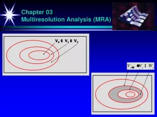
Series Expansion • In MRA, scaling function to create a series of approximations of a function or image, wavelet to encode the difference in information between different approximations • A signal or function f(x) can be analyzed as a linear combination of expansion functions
Scaling Function Set{j,k(x)} where, K determines the position of j,k(x) along the x-axis, j -- j,k(x) width, and 2j/2—height or amplitude The shape of j,k(x) change with j, (x) is called scaling function
Fundamental Requirements of MRA • The scaling function is orthogonal to its integer translate • The subspaces spanned by the scaling function at low scales are nested within those spanned at higher scales • The only function that is common to all Vj is f(x) = 0 • Any function can be represented with arbitrary precision
Refinement Equation h(x) coefficient –scaling function coefficient h(x) – scaling vector The expansion functions of any subspace can built from the next higher resolution space
Applications of wavelets • Pattern recognition • Biotech: to distinguish the normal from the pathological membranes • Biometrics: facial/corneal/fingerprint recognition • Feature extraction • Metallurgy: characterization of rough surfaces • Trend detection: • Finance: exploring variation of stock prices • Perfect reconstruction • Communications: wireless channel signals • Video compression – JPEG 2000
Useful Link • Matlab wavelet tool using guide • http://www.wavelet.org • http://www.multires.caltech.edu/teaching/ • http://www-dsp.rice.edu/software/RWT/ • www.multires.caltech.edu/teaching/courses/ waveletcourse/sig95.course.pdf • http://www.amara.com/current/wavelet.html