Download
1 / 34
340 likes | 480 Vues
The Multiwavelength Approach to Unidentified Gamma-Ray Sources. MOTIVATION: Gamma-ray sources should be multiwavelength objects. X-RAYS: Counterpart searches from observation. SPECTRUM: Pulsars? Neutron Stars? PULSATION/ROTATION: Periodicity searching.

E N D
The Multiwavelength Approach to Unidentified Gamma-Ray Sources MOTIVATION: Gamma-ray sources should be multiwavelength objects. X-RAYS: Counterpart searches from observation. SPECTRUM: Pulsars? Neutron Stars? PULSATION/ROTATION: Periodicity searching.
Gamma-Ray Pulsars 0.5-2 KeV Additional candidates: 2-100 KeV 0.1-10MeV >100 MeV >100 MeV (Thompson, 2001)
Counterpart searches from observation Concept:at some level, gamma-ray sources will have X-ray counterparts. IFthe X-ray counterpart can be found, the better X-ray position information allows deep searches at longer wavelengths. The approach:using an X-ray image of a gamma-ray source error box, eliminate most of the X-ray sources from consideration based on their X-ray, optical, and radio properties. Look for a nonthermal source with a plausible way to produce gamma rays. The classic example is Geminga. Bignami, Caraveo, Lamb, and Halpern started this search in 1983. The final result appeared in 1992 with the detection of pulsations from this isolated neutron star.
RX J0007.0+7302 (possible counterpart to 3EG J0010+7309) AX J1420.1-6049 (possible counterpart to 3EG J1420-6038/GeV J1417-6100) RX J2020.2+4026(possible counterpart to 3EG J2020+4017) RX J1836.2+5925 (possible counterpart to 3EG J1835+5918) Which sources could be the next Geminga? (O. Reimer et al., 2001)
Using X-ray source catalogue to find counterparts for INTEGRAL sources EX: Stephen et al 2005, A&A 432 L49 IBIS/ISGRI first year galactic plane survey has produced a catalogue with 123 hard X-ray sources. To find the remaining 28 objects, they have cross-correlated the ISGRI catalogue with the ROSAT All Sky Survey Bright Source Catalogue (RASSBSC). 123» 53 low mass and 23 high mass X-ray binaries, 5 AGN, pulsars, variables and a dwarf nova 75 ROSAT sources»38 low mass X-ray binaries, 13 high mass X-ray binaries, 4AGN/Clusters, 5 pulsars, 3 Cataclysmic variables and 2 other sources.— Of these sources, 10 are in the list of unidentified objects.
1. IBIS (Imager on Board of Integral Satellite): 15keV-10MeV (FOV:9°x9°), angular resolution 12' 2 planes of detector: lower: CsI array: PICsIT, 3100cm2, 200keV-10MeV front: CdTe array, ISGRI, 2600cm2, 15keV-400keV 2. SPI (Spectrometer on Integral): 20keV-8MeV (FOV:16°x16°), angular resolution 2°
The software to analyze the INTEGRAL data • INTEGRAL Off-line Scientific Analysis (OSA): • OSA is composed of the following packages: • Off-line Scientific Analysis Software (OSA_SW): 1GBytes • Instrument Characteristics (OSA_IC): 215 MBytes for IBIS, 540 MBytes for JEMX, • 340 MBytes for OMC and 1.4 GBytes for SPI • 'High-energy' Catalogue (OSA_CAT): 62 Mbytes • Test Observations, which consist of a set of data and related scripts • (OSA_TESTDATA) • **A total disk space of 3 GBytes is needed to install all available test data packages. • After running the testing scripts, the disk space required grows to 5 Gbytes.
Data Repositories On 18 Oct. 2004, all public INTEGRAL data become available both in the older and in the revised format of the Archive.
Data Repositories Aux: contains auxiliary data products received or created by Auxiliary data Preparation Cat: contains observational catalogs necessary for data analysis Ic: contains data concerning the instrumental calibrations and operational characteristics that are generated offline Idx: contains ISDC index files used for fast searching of data for selected data products Obs: contains results of Science Analysis Scw: contains the results of processing from the science window pipelines on a pre-science window basis RRRRPPPPSSSF.000 RRRR is the revolution number PPPP is the ISOC pointing number SSS is a sequence used to subdivide pointings or slews during process if required F is a flag representing the science window type (0=pointing, 1=slew, 2=non-science, values larger than 2 are unidentified)
Data Repositories • An INTEGRAL revolution of three days (about 72 hours) results in a telemetry • volume of approximately 2 Gb. This telemetry stream is processed and analyzed • At the ISDC and will result in about 17 Gb of uncompressed data products per • revolution. • raw data (4.5 Gb), which are reformatted the same information content as the • telemetry sent by the spacecraft. • prepared data (7.2 Gb), including additional timing information • corrected data (2.7 Gb), including gain corrected event energy • high-level products (2.7 Gb), which are the results of the scientific analysis in • the form of image, spectra, light curves etc. How to get INTEGRAL data http://isdc.unige.ch/index.cgi?Data+browse
Press the 'Save scw list for the creation of Observation Groups' button and Save the file with the name xxxx.list This file will be used later as input for the og_create program. Environments of the analysis data Ex: At vela2: export ROOTSYS=/disk2/HEAsoft/osa_sw-5.1/root export ISDC_ENV=/disk2/HEAsoft/osa_sw-5.1 export ISDC_REF_CAT=$REP_BASE_PROD/cat/hec/gnrl_refr_cat_0023.fits[1] export REP_BASE_PROD=the storage directory of your data my_variable=my_value; export my_variable ln –s /disk2/HEAsoft/osa_sw-5.1/INTEGRAL_packages/ic ic ln –s /disk2/HEAsoft/osa_sw-5.1/INTEGRAL_packages/idx idx ln –s /disk2/HEAsoft/osa_sw-5.1/INTEGRAL_packages/cat cat
The first step in the data analysis is creation of the Observation Group from the list of prepared Science Window Groups DOL’s you want to analyze. Data analysis For example: To create the file of the list—dith.lst scw/0044/004400540010.001/swg.fits[1] scw/0044/004400550010.001/swg.fits[1] scw/0044/004400560010.001/swg.fits[1] scw/0044/004400570010.001/swg.fits[1] Then og_create idxSwg=dith.lst ogid=isgri_gc baseDir="./" instrument=IBIS Creates a directory obs/isgri_gc with an Observation Group og_ibis.fits in it.
Image Reconstruction I. To start the analysis, move to working directory $REP_BASE_PROD/obs/isgri_gc and call the ibis_science_analysis script ? Light curve
GUI to Do the Scientific Analysis ibis_scw1_analysis and ibis_scw2_analysis work on a Science Window basis while ibis_obs1_analysis works on the Observation Group basis.
Process of Scientific Analysis Background step for Imaging Background step for Spectra Background step for Light curves Composition of the main script ibis_science_analysis.
The objects in the catalog were compiled from the following sources: • Macomb & Gehrels gamma-ray sources catalog • Liu et al. LMXB and HMXB catalogs • The 4th Uhuru catalog • Van Paradji's X-ray Binaries catalog • HEAO1 A4 catalog • BATSE observations of Piccinotti's sample of AGN • Tartarus reduced AGN data • ASCA Survey catalogs • Recent IAUCs and ATels • INTEGRAL catalogs (archive, survey, GCDE, etc.) • The IGR sources page (J. Rodriguez) • In the catalog, you will find information on the name(s) of a source, its position, and • error. Identifiers are SIMBAD-compliant and all positions are referenced. Sources in • the HTML (http://isdc.unige.ch/Data/cat) version have names that link directly to the • relevant page in SIMBAD and a position that links to the reference in ADS. The General Reference catalog and the Resulted Source list This figure presents the galactic distribution of the latest catalog's 1523 sources. The size and color of the symbols indicate approximate brightness and hardness, respectively. Symbol size is logarithmically proportional to the total ISGRI+JEM-X counting rates. Hardness is defined as (H−S)/(H+S), where H is the total ISGRI counting rate (20-200 keV), and S is the soft-band (3-10 keV) JEM-X counting rate.
Image Reconstruction II. Overview of the IMA level products
Spectral Extraction cd $REP_BASE_PROD/obs/isgri_gc fcopy “isgri_srcl_res.fits[ISGR_SRCL_RES][DETSIG >= 6.0]” specat1.fits Spectral Energy Binning Input Catalog Background Map Number of Energy Bins Parameters for Light curve extraction Energy Boundaries Time Resolution
Spectra are produced for each science window, Ex: scw/004700530010.001/isgri_spectrum.fits Results of the Spectral Extraction To achieve a better signal to noise ratio, it can be convenient to sum up spectra of a source from different science windows. cd $REP_BASE_PROD/obs/isgri_sc spe_pick group="og_ibis.fits[1]" source= "IGR J16320-4751" rootname=IGRJ16320-4751 response=$REP_BASE_PROD/ic/ibis/rsp/\ isgr_rmf_grp_0015.fits As a result two files with spectra of IGR J16320-4751 will be created: IGRJ16320-4751_sum_pha.fits contains the final average spectrum of IGR J16320-4751, while IGRJ16320-4751_single_pha2.fits stores all the original spectra of IGR J16320-4751 that were used to create the average one. In order to deal with the data from different time periods spe_pick was updated and creates now a resulting ARF for your particular dataset. It is written to IGRJ16320-4751_sum_arf.fits and IGRJ16320-4751_single_arf.fits files.
Results of the Spectral Extraction Before analyzing the average spectrum with XSPEC: fparkey 0.02 IGRJ16320-4751_sum_pha.fits SYS_ERR add=yes
Lightcurve Extraction Note that to extract the lightcurve for a source you need the Pixel Illuminated Fraction (PIF—isgri_pif.fits) map. Such a map is created during the spectral step that we have just run!! The lightcurve extraction is performed by building shadowgrams for each time and energy bin. Hence this step is time and space consuming. Note that due to CFITSIO limitations, the product of number of energy bins by number of time bins in a science window should be less than 250. ………
In case you want to re-run the analysis with different parameters, run og_create but this time with a different "ogid" parameter. This will create a new tree under obs/ogid where all the new results will be stored. If the pipeline has crashed, in general it is safer to restart your analysis from scratch removing the obs/ogid directory and restarting from the og_create step!! Rerunning the analysis|||Orz ……… Because of the group concept you cannot just delete the result you do not like and restart the pipeline. All results that were produced in the course of the analysis are linked to the group, and should be detached before you relaunch the script. To do this you can use the og_clean program, that will clean an Observation Group up to the level specified with parameter endLevel. All data structures with a level equal or prior to endLevel will be kept, while the data structure with a later level will be erased. For example, to run the spectral extraction (SPE level) you should clean from group whatever comes after the BIN_S level, as this is the level immediately preceding the spectral one. og_clean ogDOL="og_ibis.fits[1]" endLevel="BIN_S" If og_clean fails it could be due to the fact that the group was corrupted. You should try to fix it with dal_clean program dal_clean inDOL="og_ibis.fits[1]" checkExt="1" backPtrs="1" checkSum="1" and launch og_clean only afterwards.
Unfortunately the current version of og_clean is very slow!!! In some cases, if you know exactly which data structure has to be detached it would be much faster to launch dal_detach. For example if you run your analysis till SPE, or LCR level, and would like to produce a mosaic image afterwards, you do not have to clean the group, deleting all your results, but just have to detach ISGRI-SRCL-RES data structure (note that with the option "delete=y" all files with this data structure will be deleted): dal_detach og_ibis.fits[1] pattern=ISGR-SRCL-RES delete=y Rerunning the analysis|||Orz
(Cassam-Chenaї et al. 2004) The value of L in blackbody model is lower than predicted by standard cooling NS models for which luminosity is ~1034erg s-1 for a NS of a few thousand years (e.g. Tsurata 1998). Such a low luminosity could be explained by accelerated cooling process. Note that the temperature, radius and luminosity of the central point source 1WGA J1713.4- 3949 are almost identical to what is found for the central point source in SNR RX J0852.0- 4622 (also G266.2-1.2 or "Vela Junior“) adopting a distance of 1 kpc. (Becker & Aschenbach 2002; Kargaltsev et al. 2002)
An Example: 3EG J1835+5918 (O. Reimer et al., 2001) Compatible with a non-variable source of an average flux of (E >100MeV) The hard spectral index, as determined to be -1.70.06 between 70 MeV and 4GeV. The spectrum resembles the γ-ray spectra of known γ-ray pulsars like Vela or Geminga(Thompson et al. 1997).
Characteristic age: Spin-down energy: Magnetic field: Open field line voltage: The current of relativistic particles flow: year B1509-58 erg/s Crab Vela B1046-58 B0656+14 B1706-44 gauss Geminga B1055-52 B1951+32 volt s-1 J0218+4252 (Thompson, 2001)
Using X-ray source catalogue to find counterparts for INTEGRAL sources EX: Stephen et al 2006, A&A Mar. The second IBIS/ISGRI survey has produced a catalogue with 209 hard X-ray sources. To find the remaining 59 objects, they have cross-correlated the ISGRI catalogue with the ROSAT All Sky Survey Bright Source Catalogue (RASSBSC), ROSAT Faint Source Catalogue and ROSAT HRI catalogue. Compare with RASSBSC: 114 associations - Of these sources, 8 are in the list of unidentified objects. Compare with RFSC: 29 correlations - Of these sources, further 9 sources remain unidentified. Compare with ROSAT HRI catalogue: 2 unidentified sources are neither in the bright or faint source catalogues. They finally found possible identifications for nine of total 19 objects with X-ray counterparts.