Chapter 24a: Molecules in Motion Basic Kinetic Theory
110 likes | 580 Vues
Chapter 24a: Molecules in Motion Basic Kinetic Theory. Homework: Exercises (a only) : 4, 5, 6, 8, 10. Kinetic Model of Gases. Motion in gases can be modeled assuming Ideal gas Only contribution to energy of gas is the kinetic energy of the molecules (kinetic model)

Chapter 24a: Molecules in Motion Basic Kinetic Theory
E N D
Presentation Transcript
Chapter 24a: Molecules in MotionBasic Kinetic Theory Homework: Exercises (a only) : 4, 5, 6, 8, 10
Kinetic Model of Gases • Motion in gases can be modeled assuming • Ideal gas • Only contribution to energy of gas is the kinetic energy of the molecules (kinetic model) • Basic Assumptions of Kinetic Model: 1. Gas consists of molecules of mass, m, in random motion 2. Diameter of molecule is much smaller than average distance between collisions • Size negligible 3. Interaction between molecules is only through elastic collisions • Elastic collision - total kinetic energy conserved
Pressure and Molecular Speed • Bernoulli’s Derivation* - • Assumptions • Collection of N molecule, behaving as rigid spheres • Random velocities in volume, V • Consider movement in x direction (normal to a wall) • Heading toward wall is positive x • Fraction with velocity u + du specified by density function, f(u), where • dN(u)/N = f(u) du • f(u) probability velocity between u ® u +du • No need to define this function further at this point *slightly different approach than book
Pressure and Molecular Speed • Bernoulli’s Derivation - • Kinematics • In time dt, only molecules striking wall are those with positive velocity (u>0) between u and u+du • Assumes initial distance ≤ udt • # of Molecules striking wall during dt are those within volume V=Audt at t= 0 with right velocity N/V(f(u)du))isN/Vf(u) Audt du • Momentum change with each collision is Dp= mu - (-mu) = 2mu. Incremental momentum change is:
Pressure and Molecular Speed • Bernoulli’s Derivation - • Pressure (P) = force/area, so • Integrating over all + velocities since only they contribute to pressure on wall
Consequences of Kinetic Model of Equation of State (PV = 2/3 Ek) • Kinetic model looks a lot like Boyle’s law (PV = constant @ constant T) • Since the mean square speed of molecules should only depend on temperature, the kinetic energy should be consatnt at constant T • In fact if NRT = 2/3 Ek, Kinetic Model is the ideal gas equation of state • Since Ek = 0.5Nmc2,it follows that <c2>1/2a T1/2 and <c2>1/2a (1/m)1/2 {<c2>1/2 is the root mean square speed} • The higher the temperature, the faster the mean square speed • The heavier the molecule, the slower the mean square speed
Distribution of Speeds, f(u)du • Earlier didn’t define f(u) exactly • James Clerk Maxwell (1860) derived distribution • Key assumption: probability of particle having a velocity component in one range (u +du) independent of having another component in another range • If this is true, the distribution function, F(u,v,w), is the product of components in each direction F(u,v,w) = f(u)f(v)f(w) • Not fully justified until advent of quantum mechanics • Law proved by Boltzmann in 1896 • Verified experimentally • If v is the speed of a molecule, • Features of distribution • Narrow at low temperatures, broadens as T increases • Narrow for high molecular masses, broadens as mass decreases
Using Maxwell Distribution • Evaluating Maxwell distribution • Over narrow range, Dv,evaluate f(v) Dv • Over wide range, numerically integrate, • Mean speed of particle • Mean speed (not mean root speed) is calculated by integrating the product of each speed and the probability of a particle having that speed over all possible speeds
Molecular Speed Relationships • Root mean speed, c, c = (3RT/M)0.5 • Mean speed, c , c = (8RT/πM)0.5 • Most probable speed, c* • Maximum of Maxwell distribution, i.e, df(v)/d(v) = 0 c* = (2RT/M)0.5 • Most probable speed = (π/4)0.5 x mean speed = 0.886 c • Relative mean speed, crel,speed one molecule approaches another • Range of approaches, but typical approach is from side
Collisions • Collision diameter, d - distance > which no collision occurs, i.e., no change in p of either molecule • Not necessarily molecular diameter, except for hard spheres • N2, d = 0.43 nm • Collision frequency, z - number of collisions made by molecule per unit time z = s x crel x N s = collision cross section = πd N = # molecules per unit volume = N/V crel = relative mean speed • For ideal gas, in terms of pressure , z = (s crel p)/kT • As T increases, z increases because the rel. mean speed a T1/2 • As p increases, z increases because the # of collisions a density of gas a N/V • N2 at 1 atm and 25°C, z = 5 x 10⁹ s-1
Collisions • Mean free path, l - average distance between collisions l = mean speed ¸ collision frequency • Doubling p halves l • At constant V, for ideal gas, T/p is constant so l independent of T • l(N2) = 70 nm • At 1 atm & RT, most of the time, molecules far from each other • Collision Flux, zw - # collisions per unit time and area zw = p/(2πmkT)0.5