Download
1 / 38
380 likes | 561 Vues
Positive Influence Dominating Set and Beyond. My T. Thai @ UF. Spread of Influence. Online Social Networks (OSNs) have been exploited as a platform for spreading INFLUENCE Opinions Information Viral marketing Innovation Political campaigns…. Spread of Influence (Examples).

E N D
Positive Influence Dominating Set and Beyond My T. Thai @ UF
Spread of Influence • Online Social Networks (OSNs) have been exploited as a platform for spreading INFLUENCE • Opinions • Information • Viral marketing • Innovation • Political campaigns… My T. Thai mythai@cise.ufl.edu
Spread of Influence (Examples) • Major movie studios place trailers for their movies on Facebook; • US presidential candidates ran online political campaigns on YouTube; • Individuals and amateur artists promote their songs, artwork, and blogs through these sites My T. Thai mythai@cise.ufl.edu
Information Propagation & Myths • It is widely believed that through the “word of mouth” effects, influence will spread widely and quickly throughout the network. My T. Thai mythai@cise.ufl.edu
Information Propagation - The Truth • M. Cha et al. WWW’09, Propagation in Flickr. • Howwidely does information propagate in the social network? • Not widely – within two yards • Howquickly does information propagate? • Not quickly, it takes a long time. The average delay in information propagation across social links is about 140 days!!!
Fast Influence Spreading Problem • Given • Network G=(V, E). • The maximum number of propagation hops d. • Goal • Spread the influence into the whole network within d hops (e.g. dominate a particular market) • Question • What is the minimum set of individuals to target at? My T. Thai mythai@cise.ufl.edu
What’s next? • Influence Propagation Model • Direct Influence: number of hop d=1 • Generalized Dominating Set • Tractability & Approximation Algorithms on • General Graphs • Bounded Degree Graphs • Power-law Graphs • Trees • Multiple-hop Propagation • Hardness of approximation • Selection Algorithm My T. Thai mythai@cise.ufl.edu
I. Models of Influence 1 • General operational view: • A social network is represented as a graph, with each person (customer) as a node • Nodes start either active or inactive • An active node may trigger activation of neighboring nodes • Monotonicity assumption: active nodes never deactivate • First mathematical models • [Schelling '70/'78, Granovetter '78] 0 1 1 1 0 1 2 2
I. Model of Influence • Major models: Linear Threshold and Independent Cascade • Linear threshold: Each node v has a threshold wvv is activated if there are ≥ tvactive neighbors. • Independent Cascade: An active node u activates its neighbor v independently with probability puv. • Our models: Linear Threshold • v is activated if there are ≥ v d(v)active neighbors. • d(v): degree of v; 0< v < 1. My T. Thai mythai@cise.ufl.edu
II. Direct Influence in Networks (d=1) My T. Thai mythai@cise.ufl.edu
Positive Influence Dominating Set(PIDS) 1 • Given: A graph G=(V, E) and a single constant 0< < 1 . A node v V has threshold d(v). • Problem: Find minimum set P V, so that after d=1 hop, all nodes are activated. • Intuition: Half of my friends use Iphone, why shouldn’t I? 0 1 1 1 0 0 1 1 My T. Thai mythai@cise.ufl.edu
Generalized Dominating Set (GDS) • The threshold function might not be linear • log d(v), d(v), etc. • Characteristics of a threshold function: • A node v is activated if ≥ rv (d(v)) active neighbors. • Monotone increasing function • dominating function. My T. Thai mythai@cise.ufl.edu
Problems in GDS • Dominating set: rv (x) = 1. • k-tupledominating set: rv (x) = k. • Positive influence dominating set: rv (x) = x. • Fixed threshold model: rv (x) = tv . • … • GDS capture the dynamic aspect of networks. • More neighbors Threshold Increase and vice versa. My T. Thai mythai@cise.ufl.edu
Properties of Dominating Set • Total: Even nodes in the dominating set have to dominate themselves • Connected: The induced subgraph is connected • k-connected: The induced subgraph is k-vertex connected (cannot disconnect the graph by deleting k-1 vertices.) • and combinations • Total connected • k-connected total My T. Thai mythai@cise.ufl.edu
Generalized DS and MORE… • TOTAL GDS (T-GDS) • CONNECTED GDS ( C-GDS) • k-CONNECTED GDS (kC-GDS) • TOTAL CONNECTED GDS (TC-GDS) • k-CONNECTED TOTAL GDS (kCT-GDS) My T. Thai mythai@cise.ufl.edu
Bad News • All domination problems in all mentioned classes • Cannot be approximated within ln - O(lnln ), unless P = NP. • Cannot be approximated within(1/2 - ) ln |V|, unless NP DTIME(no(log log n) ) where is the maximum degree of G=(V,E). • Cannot be approximated within lnB- O(lnlnB), unless P = NP, in graphs with degrees bounded by B • APX-hard even in Power-law networks My T. Thai mythai@cise.ufl.edu
Good News • Problems in GDS: approximated within H(2). • Problems in T-GDS: approximated within H(). • Problems in C-GDS: approximated within H(3). • Problems in TC-GDS: approximated within H(2). • In power-law networks: PIDS-like problems (r(x) >x for some constant ) problems are approximated within a constant factor • In trees: Optimal solution in linear time. H(n)=1+1/2+…+1/n is the harmonic function. My T. Thai mythai@cise.ufl.edu
Inapproximability e1 • Typical road map: Reduction from Set Cover • But, involve many tweaking of Feige’s (1-o(1)) ln n threshold proof. x'1 x1 S1 e2 . . . . . . . . S2 e3 x'i xi S3 e4 . . . . . . . . . . . . e5 S|S| xt . . . . x't e|U| D’ D S U My T. Thai mythai@cise.ufl.edu
Feige’s reduction • Reduction from MAX 3SAT-5 to k-provers proof system. • k provers : k binary code words of length l, weight l/2 and Hamming distance at least l/3. • The provers select randomly l/2 clauses and l/2 variables. • Acceptance predicate: • Weak: at least one pair of provers is consistent. • Strong: every pair of provers is consistent. My T. Thai mythai@cise.ufl.edu
Feige’s Reduction: Construction • A partition system B(m,L,k,d) has the following properties. • There exists a ground set B of mdistinct points. • There is a collection of L distinct partitions p1,…,pL. • For 1≤i≤L, partition pi is a collection of k disjoint subsets of B whose union is B. • Any cover of the m points by subsets that appear in pairwise different partitions requires at least d subsets. • R=(5n)l : Number of random strings. • r↔Br(m,L,k,d): m=nΘ(l), L=2l, d=(1-2/k)k∙ln(m), Q=nl/2(5n/3)l/2 (questions to Pi). • Universal U = Unions of all Br • Collection S = Subsets S(q,a,i): question q, answer a, proveri. • Q=nl/2(5n/3)l/2(questions to proveri). My T. Thai mythai@cise.ufl.edu
Feige’s Hidden Parameters • Number of subsets in S? • |S| Q 22l • Maximum size of a subsets? • m 3l/2 : For each iand q, there are at most 3l/2 random strings such that the verifier makes query q to the proveri. • Maximum frequency of a point/element? • F k 2l l: Each partition contains k copies of a point, and a subsets contains at most 2l subsets from a same partition. My T. Thai mythai@cise.ufl.edu
Hardness Ratio and Suf. cond. • The hardness ratio • (1-4/k) ln m [ ln m vs. ln (mR +Q 22l) ] • Sufficient conditions: • l >1/c (5 log k+2log ln m) • To get (1-) ln n: Feiget set m = (5n)2l/ very large Number of vertices My T. Thai mythai@cise.ufl.edu
Set Cover to GDS e1 • Hardness ratio from our reduction: • where |D| ~ • Feige settings give hardness ratio ~ 1 x'1 x1 S1 e2 S2 e3 x2 x'2 S3 e4 . . . . . . . . . . . e5 S|S| . . . . x't xt e|U| D’ D S U My T. Thai mythai@cise.ufl.edu
Hardness of GDS, T-GDS,… • Optimal setting for our reduction • m = (5n)l(1-) • Hardness ratio > (1/2 - ) ln |V| • We make D a clique total, k-connected. My T. Thai mythai@cise.ufl.edu
Hardness of GDS, T-GDSin Bounded Graphs e1 • In graph with degrees bounded by B. We use Trevisan [STOC’01] settings for bounded set cover. • m = B/poly log B. • New issue: Keep degreeof vertices in D bounded. • Possible by choosing|D| = mR/B ln2B. • Hardness: lnB - O(lnln B), unless P = NP hardness ln - O(lnln ) x'1 x1 S1 e2 S2 e3 x2 x'2 S3 e4 . . . . . . . . . . . e5 S|S| . . . . x't xt e|U| D’ D S U My T. Thai mythai@cise.ufl.edu
Bounded degree: kC-GDS • Issue: Cannot make |D| a clique (bounded degree) • Solution: Connect |D| using a 2k-Ramanujan graph |D| has vertex expansion at least k. My T. Thai mythai@cise.ufl.edu
Approximation Algorithms • GDS, T-GDS reduction to • C-GDS, TC-GDS: Greedy algorithm using analysis technique for non-supmodular potential function. [ Du et al., SODA 2008] My T. Thai mythai@cise.ufl.edu
PIDS-like DS in Power-law Graphs • PIDS-like: rv(x) > x • Long tails make it “easier” to approximate the optimal solution • Primal-Dual fitting to give Lower bound on size of PIDS-like DS. My T. Thai mythai@cise.ufl.edu
PIDS-like DS in Power-law Graphs • Objective of Dual feasible solution lower bound for Primal • Strategy: Force all yu dual variables to have a same value . Optimize using degree distribution to give the best lower bound. My T. Thai mythai@cise.ufl.edu
PIDS-like DS in Power-law Graphs • Power-law distribution: • y vertices have degree x: • is log-log growth rate network characteristics • Size of networks: My T. Thai mythai@cise.ufl.edu
PIDS-like DS in power-law Graphs • Results: • All DS have size at least (|V|)!!! • Trivial constant approximation algorithm. • Agree with the NOT WIDELY propagation observation • Require a large number of initial target to propagate to the whole networks. My T. Thai mythai@cise.ufl.edu
Optimal Solutions in Trees • kC-GDS: Optimal solutions are on non-leaf nodes! Trees are really easy !!! My T. Thai mythai@cise.ufl.edu
III. Multiple-hop Propagation My T. Thai mythai@cise.ufl.edu
Approximability • Hardness of Approximation • (1-o(1)) ln n for d < 4 • for d 4 • Approximation: • Constant factor approximation algorithm in power-law networks • Initial set is again (|V|)!!! My T. Thai mythai@cise.ufl.edu
Efficient Heuristics for Large Scale Networks VirAds-Fast-Spreading Algorithm • A priority queue of nodes: priority = # affected vertices + #affected edges. • Pickup vertex with highest priority • Recalculate priority, and select the vertex if the new priority is still the highest, repeat otherwise • Update the number of activated vertices with the selected node • Lazy update: Update priority for only vertices that are “affected” by the selected vertex. Repeat! My T. Thai mythai@cise.ufl.edu
Heuristics for Large Scale Networks • Datasets: Facebook • New Orleans City: 90 K vertices, ~4M edges. • Orkut social network: 3 M vertices, 220 M edges • Competitors: • Max degree selector • Virads: One-hop greedy selector • Virads-Full-Spreading: • Expensive multi-hop greedy • Cannot run for large networks (e.g. Orkut) My T. Thai mythai@cise.ufl.edu
Experiments Results • Running time on Orkut (220 M edges): • Virads-Fast-Spreading: Few minutes • Virads-Full-Spreading: >> weeks. • Quality is on par with the expensive multihop-greedy. My T. Thai mythai@cise.ufl.edu
Thank you for listening! Spheres of influence are now the measure of power in human relationships. My T. Thai mythai@cise.ufl.edu