Closure Properties of Regular Languages
250 likes | 881 Vues
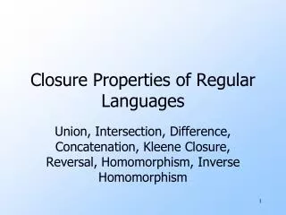
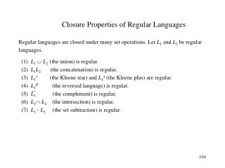
Closure Properties of Regular Languages. Re gular languages are closed under many set operations. Let L 1 and L 2 be regular languages. (1) L 1 L 2 (the union) is regular. (2) L 1 L 2 (the concatenation) is regular.

Closure Properties of Regular Languages
E N D
Presentation Transcript
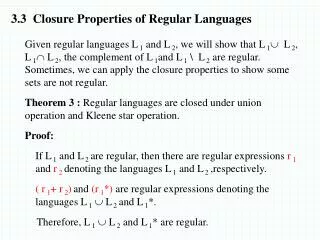
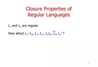
Closure Properties of Regular Languages • Regular languages are closed under many set operations.Let L1 and L2 be regular • languages. • (1) L1 L2 (the union) is regular. • (2) L1L2 (the concatenation) is regular. • (3) L1 (the Kleene star) and L1+ (the Kleene plus) are regular. • (4) L1R (the reversed language) is regular. • (5) L1 (the complement) is regular. • (6) L1L2 (the intersection) is regular. • (7) L1 - L2 (the set subtraction) is regular.
Proof of the Closure Properties • We can either use regular grammars, FA, or regular expressions for the simplicity of the proof. • Let r1 and r2 be regular expressions that, respectively, express the languages L1 and L2 . • Clearly, r1 + r2 is a regular expression which denotes the union of two languages L1 and L2, respectively, denoted by r1 and r2. Since every regular expression denotes a regular language, L1 L2 is regular. • We can also constructively prove this property as follows; let G1= ( VN1, VT1, P1, S1 ) and G2 = ( VN2, VT2 , P2, S2) be regular grammars that generate L1 and L2 , respectively. Without loss of generality, assume that VN1 and VN2 are disjoint, i.e., VN1VN2 = . Otherwise, we can always convert the given grammars to the ones that satisfy such property. Construct a regular grammar G with production rules S S1 | S2 and all the rules in P1 and P2. Clearly, L(G) = L1 L2 . • (2) Clearly r1r2 is a regular expression which denotes the language L1L2, which means L1L2 is regular. • (3) Let r1 be regular expression for L1. Clearly, (r1)* is regular expression for L1 Since L1+ = L1 - {}, by property (7) that will be proved, L1+ is regular.
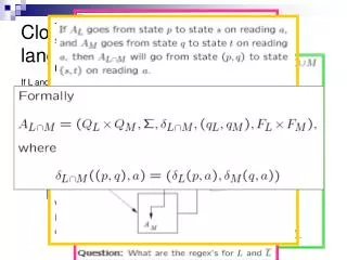
Add a new accepting state a a a start a a b start a a b b a b b start b a a Let the new accepting state be the start state, reverse the direction of all the edges, and the old start state be the only accepting state. a b a b b Proof of the closure Properties (cont’ed) (4) Suppose that the following FSA M1 accepts L1. We modify M1 as shown below. Clearly, the resulting automaton recognizes the reversed language of L1.
Proof of the Closure Properties (cont’ed) • You can also prove part (4) using a regular grammar G1using another form of regular grammars, where the production rules are restricted to the form either A Bx, or A x, where A and B are arbitrary nonterminal symbols, and x is a string of terminal symbol, or . (Recall that we chose to restrict to A xB, or A x.) If we reverse the right side of each production rule, then the resulting grammar G generates L1R . • (5) As for part (4), we modify the finite transition graph M1of an automaton that recognizes L1 as follows. • Add the dead state, if it is not shown in the transition graph. (Recall that we usually do not show the dead state for convenience.) • Change accepting states to non-accepting states and non-accepting states to accepting states. • (6) SinceL1 L2= L1 L2 = L1 L2 , and regular language are closed under union and complementation (properties (1) and (5) above), L1 L2 is regular. • (7) Since L1 - L2 = L1 L2 , it is regular by properties (5) and (6)above.
Properties of Context-free Languages • Let L1 and L2 be CFL’s. • (1) L1 L2 (the union) is CFL. • (2) L1L2 (the concatenation) is CFL. • (3) L1 * (the Kleene star) and L1+ (the Kleene plus) are CFL. • (4) L1R (the reversed language) is CFL. • (5) L1 L2 (the intersection) is not necessarily CFL. • (6) L1 (the complement) is not necessarily CFL.
Proof of the Context-free Language Properties • LetG1 = ( VN1, VT1, P1, S1 ) and G2 = ( VN2, VT2 , P2, S2 ) be CF grammars that • generate L1 and L2 , respectively. Without loss of generality, assume that VN1 and • VN2 are disjoint, i.e., VN1 VN2 = . (Otherwise, we can modify them.) • (1) Construct a CFG G by merging the rules of grammars G1 and G2 and adding new rules S S1 | S2. (This is the same technique for regular languages.) • (2) Construct a CFG G by merging the rules of G1 and G2 and adding a new rule • S S1S2. • (3) For L1 * add rules S S1S | in grammar G1. For L1+ add rules S S1S | S1 • ,where S is new start symbol. • (4) Construct a CFG from G1 by changing each rule A to A R, i. e., reverse right side of each production rule.
Proof of the Context-free Language Properties (cont’ed) • (5) We know that L1 = {a ib ic j i, j 0 } and L2 = {a k b nc n k, n 0 } • are CFL’s. But L1 L2 = {a i b i c i i 0 } is not CFL. • (6) Suppose that CFL’s are closed under complementation. Since CFL’s are • closed under union (property (1)), and L1 L2 = L1 L2 , which implies • CFL’s are closed under intersection. This contradicts to the proven fact of • property (5).
Minimizing the Number of -Production Rules • Theorem. Given an arbitrary CFG G, we can construct a CFG G´ such that • L(G) = L(G´) and if is not in L(G), then G´ dose not have - production rule. • If L(G), then S is the only -production rule of G´. • Proof (an algorithm). Let G = (VT, VN, P, S), and let A, B VN. We construct a CFG G´ = (VT ,VN ,P´, S) from G by the following steps. • (1) Find the set W of all nonterminals of G which derive as follows; • W0 = {A| A VN and A is in P}; • Do Wi+1 = Wi {A | A VN and A is in P, for some Wi +}; • until (Wi+1 = Wi); • W = Wi; //W contains all nonterminal symbols from which can be derived. • (2) Delete all -production from P. Call this new set of productions P1. • (3) Modify P1 to P´ as follows: If a production A is in P1, then put the rules A and A into P´, for all ( ) which are obtained from by deleting one or more nonterminals in the set W constructed by step (1). • (4) If S is in W, then add S in P´.
Minimizing the Number of -Production Rules (example) Convert the following CFG G to another CFG G´ such that L(G) = L(G´) and G´has the smallest possible number of -production rules. G: S ADC | EFg A aA | D FGH | b C c | E a F f | G Gg | H H h | Computing W: W0 = {A, C, F, H} W1 = W0 {G} = {A, C, F, G, H} W2 = W1 {D} = {A, C, D, F, G, H} W3 = W2 {S} = {A, C, D, F, G, H, S} W4 = W3 {} = {A, C, D, F, G, H, S} P1:S ADC | EFg A aA D FGH | b C c E a F f G Gg | H H h P´:S ADC | AD | AC | DC | A | D | C | | EFg | Eg A aA | a D FGH | FG | FH | GH | F | G | H | b C c E a F f G Gg | g | H H h
Eliminating Useless Symbols from a CFG • Lemma 1. Given a CFG G = (VT , VN , P, S), we can construct an equivalent CFG G´ = (VT , V´N , P´, S), such that every nonterminal symbol A in V´N derives a string x (VT)* • Proof. Let OLDV and NEWV be sets of nonterminals, and A be an arbitrary nonterminal. We construct V´N and P´ as follows. • OLDV = ; NEWV = {A | A w is in P for some w (VT)* }; • while (OLDV NEWV) do • { • OLDV = NEWV; • NEWV = OLDV {A | A for some in (VT OLDV)*}; • } • V´N = NEWV; P´ = {A | A is in P and (V´N VT)*};
Eliminating Useless Symbols from a CFG(cont’ed) Lemma 2. Given a CFG G = (VT,VN, P, S), we can construct an equivalent CFG G´ = (V´T ,V´N , P´, S), such that, for each symbol X V´T V´N , the start symbol derives X, for some , (V´T V´N)*, i.e., S can derive a sentential form (a string of terminals and nonterminals) which contains symbol X. Proof. The following algorithm computes V´T, V´N and P´. (1) Let V´T and V´N be the empty sets. (2) Put S into V´N. (3) If A VN is put into V´N and A 1 |2 | .... n , then all nonterminals in i, 1 i n, are put into V´N and all terminals in are put into V´T. (4) Repeat (3) until there is no symbol to be added to V´N . (5) Let P´ contain all the productions in P except for the ones which have a symbol not in V´T V´N.
Eliminating Useless Symbols from a CFG(cont’ed) • Theorem. Given arbitrary CFG G = (VT , VN , P, S), we can construct an • equivalent CFG G´ = (V´T , V´N , P´, S), such that, • (1) for each A V´N , A (V´)*T (i.e., A derives a terminal string or ), and • (2) for each X V´T V´N , S X, for some , V´N (V´)*T, • (i.e., the start symbol can drive a sentential form which contains X). • Proof. Use Lemmas 1 and 2.
Eliminating Useless Symbols from a CFG(example) Example. Eliminate useless symbols from the following CFG G. G: S AD | EFg A aGD D FGd C cCEc E Ee F Ff | G Gg | g H hH | h Step 1: Apply Lemma 1 to find the set of nonterminals V´N such that every nonterminal symbol in V´N derives a string x (VT)*. OLDV = {}; NEWV = {F, G, H} OLDV = NEWV; NEWV = OLDV {D} = {D, F, G, H}; OLDV = NEWV; NEWV = OLDV {A} = {A, D, F, G, H}; OLDV = NEWV; NEWV = OLDV {S} = {A, D, F, G, H, S}; OLDV = NEWV; NEWV = OLDV { } = {A, D, F, G, H, S}; V´N = NEWV = {A, D, F, G, H, S} Find the set of rules P´ . P´: S AD A aGD D FGd F Ff | G Gg | g H hH | h
P´: S AD A aGD D FGd F Ff | • G Gg | g H hH | h • Step 2: Find the set of symbols V´ = V´T V´N such that each symbol in V´ can be derived starting from S. • V´T = V´N = {}; // initialize with empty set • V´N = V´N {S} V´T = V´T {} • V´N = V´N {A, D} = {S, A, D} V´T = V´T {} • V´N = V´N {G, F} = {S, A, D, G, F} V´T = V´T {a, d} ={a, d} • V´N = V´N {} = {S, A, D, F, G} V´T = V´T {a, d} ={a, d, g, f} • V´N = V´N {} = {S, A, D, F, G} V´T = V´T {} ={a, d, g, f} • Cleaned set of rules: • P´: S AD A aGD D FGd F Ff | • G Gg | g
Eliminating Useless Symbols from a CFG (cont’ed) • Remark: Notice that applying Lemma 2 first and then Lemma 1 may fail to • eliminate all useless productions. • Example. Consider grammar with rules P = {S AB | a A a} • By applying Lemma 1 first, we have P = {S a A a }, then applying • Lemma 2, we have P = {S a }. • However, if we apply Lemma 2 first, we have P = {S AB | a A a }. • Then applying Lemma 1, we have P = {S a A a }, which still has a • useless production.
man entered room with picture A man entered room the a A the with picture a Ambiguous Context-free Grammars • There are two kinds of ambiguities in a language. • Lexical ambiguity (or semantic ambiguity): A symbol or an expression has more than one meaning (e.g., story, saw). • Syntactic ambiguity (or structural ambiguity): An expression can be parsed in two different ways. A CFG is ambiguous if the language has a string for which there are more than one parse tree. For a given context-free grammar G and a string x, the parse tree shows how x is derived with the rules of G (see an example on the next slide). In programming language different parse trees give different object codes. In this course we will only study syntactic ambiguity of context-free grammars. Example 1 (in natural language). “A man entered a room with a picture” can be interpreted in two different ways.
S S S S S S A S S S S A p r A A A A q r p q Figure (a) Figure (b) Ambiguous Context-free Grammars (cont’ed) • Example 2 (in formal language). The following context-free grammar is ambiguous, because it • has two parse trees shown in Figures (a) and (b) below for string p q r. • G: S SSSSSA A pqr
S S ) ) ( ( S S S S A ( ) A ) S S ( S S p r A A A A p q q r Figure (b). ((p q ) r) Figure (a) (p (q r)) Some Techniques for Designing Unambiguous CFG (1) Use parenthesis such that each derivation tree generates unique string. Notice that this technique changes the language by introducing new terminal symbols, the parentheses. Example: Ambiguous G1 : S SSSSSA A pqr Unambiguous G2 : S (SS)(SS)(S) A A pqr
S S S b S b S b S S b A S b c b A c c Some Techniques for Designing Unambiguous CFG • (2) Modify the production rules that cause the ambiguity. • Examples: (a) Grammar G3 below is clearly ambiguous grammar because it can • either generate left side b first and then right side b or vice versa for string bcb. • Grammar G4 doesn’t have this possibility because it generates left side b’s first, • if any. Ambiguous G3 : S bSSbc • Unambiguous G4 : S bSA A Abc Figure (a). Ambiguity of G3 Figure (b). Unambiguous G4.
Some Techniques for Designing Unambiquous CFG(cont’ed) • (b) The following grammar G5 is ambiguous, since it can generate in two ways. • We eliminate this possibility by applying the technique of reducing -production • rules. Grammar G6 is the result. • G5 : S BD B bBc D dDe • G6 : S BD B bBcbc D dDede • (c) Grammar G1 can be modified in two different ways to make it unambiguous. • Notice that for G7 we used the same technique for Example (a) above. • G7 : S ASASSA A pqr • G8 : S DSD D C DC C CA A pqr • For G8 we set up a precedence rule such that , if any, is derived (by S) first, then • (by D) and in that order from the top of the parse tree. The later an operator is • derived the higher precedence it has over the others.
Known facts about ambiguous context-free grammars. • There is no algorithm that can tell whether an arbitrary CFG is ambiguous or not. • There is so called inherently ambiguous context-free languages for which every CFG is ambiguous. Here is an example. • {anbncmdm n, m 1} {anbmcmdn n, m 1}. • There is no algorithm that can convert an arbitrary ambiguous CFG, which is not inherently ambiguous, to an unambiguous one.
Normal Forms of Context-free Grammars When we investigate context-free grammars and their languages, sometimes it is convenient to make the right side of each production rule meet certain form. Such form is called normal form. There are two normal forms for context-free grammars; Chomsky Normal Form(CNF) and Greibach Normal Form(GNF). Let G = (VN, VT, P, S) be a context-free grammar. Grammar G is in CNF, if all the production rules of the grammar are of the form A BC or A a, where A, B, CVN, aVT. A context-free grammar is in GNF, if every production rule of the grammar is of the form A a, where A VN , aVT , and (VN)*. Notice that is a string of nonterminal symbols or a null string. We can show that every context-free grammar whose language does not contain can be converted to CNF and GNF. (Recall that we can eliminate all -production rules from a given context-free grammar, if its language does not contain .) The following example shows how to convert a context-free grammar to CNF. We can easily generalize the idea. Converting a context-free grammar to GNF is quite involved (see the text Chapter 6). We shall not study the proof.
Converting a Context-free Grammar to CNF(example) • Suppose that a context-free grammar has a production rule A aBCDbE, which is not in CNF. We introduce new nonterminal symbols and production rules in CNF such that A can derive the right side string aBCDbE as follows; • A A1B1 A1 a // and we let B1 derive BCDbE as follows; • B1 BC1 // and we let C1 derive CDbE as follows; • C1 CD1 // and we let D1 derive DbE as follows; • D1 DE1 // and we let E1 derive bE as follows; • E1 F1EF1 b // and we let E1 derive bE as follows; Example. Convert the following context-free grammar to CNF. S AaBCb A abb B aC C aCb | ac Answer: S AA1 A1 A2A3 A2 a A3 BA4 A4 CA5 A5 b A B1B2 B1 a B2 B3B4 B3 b B4 b B C1C C1 a C D1D2 | E1E2 D1 a D2 CD3 D3 b E1 a E2 c