

SlideServe
Menu
Préférences
© SlideServe · v2026

SMOKERS

owena avatar
3 diapositives · 240 Views · Jul 30, 2014

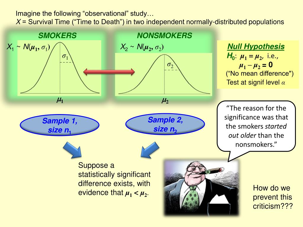
Imagine the following “observational” study… X = Survival Time (“Time to Death”) in two independent normally-distributed populations . SMOKERS. NONSMOKERS. X 1 ~ N ( μ 1 , σ 1 ). X 2 ~ N ( μ 2 , σ 2 ). Null Hypothesis H 0 : μ 1 = μ 2 , i.e., μ 1 – μ 2 = 0
SMOKERS - slide 1
01 / 3SMOKERS
1 / 17

Télécharger la présentation

SMOKERS
Une image / un lien ci-dessous est fourni (tel quel) pour télécharger la présentation

Politique de téléchargement : le contenu du site vous est fourni TEL QUEL pour votre information et votre usage personnel ; il ne peut être vendu, concédé sous licence ni partagé sur d’autres sites sans l’accord de son auteur.Le contenu vous est fourni TEL QUEL, pour votre information et votre usage personnel uniquement. Téléchargez la présentation en cliquant sur ce lien. Lors du téléchargement, si vous ne parvenez pas à télécharger une présentation, l’éditeur a peut-être supprimé le fichier de son serveur.Pendant le téléchargement, si vous ne parvenez pas à obtenir une présentation, le fichier a peut-être été supprimé par l’éditeur.

F I N

Plus de contenu associé

Transcription de la présentation
  1. Imagine the following “observational” study… X = Survival Time (“Time to Death”) in two independent normally-distributed populations SMOKERS NONSMOKERS X1~ N(μ1, σ1) X2 ~ N(μ2, σ2) Null Hypothesis H0: μ1 = μ2, i.e., μ1 – μ2= 0 (“No mean difference") Test at signif level α σ1 σ2 1 2 “The reason for the significance was that the smokers started out older than the nonsmokers.” Sample 2, size n2 Sample 1, size n1 Suppose a statistically significant difference exists, with evidence that μ1 < μ2. How do we prevent this criticism???

  2. Now consider two dependent (“matched,” “paired”) populations… X and Ynormally distributed. POPULATION 1 POPULATION 2 X ~ N(μ1, σ1) Y ~ N(μ2, σ2) Null Hypothesis H0: μ1 = μ2, i.e., μ1 – μ2= 0 (“No mean difference") Test at signif level α σ1 σ2 1 2 Classic Examples: Twin studies, Left vs. Right, Pre-Tx (Baseline) vs. Post-Tx, etc. Common in human trials to match on Age, Sex, Race,…         By design, every individual in Sample 1 is “paired” or “matched” with an individual in Sample 2, on potential confounding variables. … etc…. … etc….

  3. Now consider two dependent (“matched,” “paired”) populations… X, and Ynormally distributed. POPULATION 1 POPULATION 2 X ~ N(μ1, σ1) Y ~ N(μ2, σ2) Null Hypothesis H0: μ1 = μ2, i.e., μ1 – μ2= 0 (“No mean difference") Test at signif level α σ1 σ2 D= 1 2 Classic Examples: Twin studies, Left vs. Right, Pre-Tx (Baseline) vs. Post Tx, etc. Common in human trials to match on Age, Sex, Race,…         NOTE: Sample sizes are equal! … etc…. … etc…. Sample 2, size n Sample 1, size n Since they are paired, subtract! Treat as one sample of the normally distributed variable D = X – Y.