Download
1 / 63
640 likes | 838 Vues
A long standing puzzle General remarks on the measurement method A rotation-invariant formalism to measure vector polarizations and parity asymmetries Quarkonium polarization Heavy Ion applications. New probes for QGP: quarkonium polarisation at LHC and AFTER. Jo ão Seixas – CERN

E N D
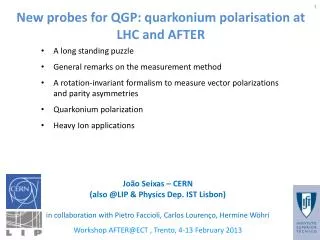
A long standing puzzle General remarks on the measurement method A rotation-invariant formalism to measure vector polarizations and parity asymmetries Quarkonium polarization Heavy Ion applications New probes for QGP: quarkonium polarisation at LHC and AFTER João Seixas – CERN (also @LIP & Physics Dep. IST Lisbon)in collaboration with Pietro Faccioli, Carlos Lourenço, Hermine Wöhri Workshop AFTER@ECT , Trento, 4-13 February 2013
A varied menu for the LHC (and AFTER) • Measure polarization = determine average angular momentum composition of the particle, through its decay angular distribution • It offers a much closer insight into the quality/topology of the contributing production processes wrt to decay-averaged production cross sections • Polarization analyses are particularly important to (for example): • understand still unexplained production mechanisms [J/ψ, χc,ψ’, , χb] • characterize the spin of newly (eventually) discovered resonances[X(3872), Higgs, Z’, graviton, ...] • Understand the properties of dense and hot matter
Task list One assumes that the production of quark-antiquark states can be described using perturbative QCD, as long as we “factor out” long-distance bound-state effects An inescapable prediction of the semi-perturbative approach (NRQCD) is that “high” pT quarkonia come from fragmenting gluons and are fully tranversely polarized Despite good success in describing cross sections...
Task list One assumes that the production of quark-antiquark states can be described using perturbative QCD, as long as we “factor out” long-distance bound-state effects An inescapable prediction of the semi-perturbative approach (NRQCD) is that “high” pT quarkonia come from fragmenting gluons and are fully tranversely polarized The first comparisons with data were not promising… NRQCD factorizationBraaten, Kniehl & Lee, PRD62, 094005 (2000) J/ψ@1.96TeV CDF Run II CDF Coll., PRL 99, 132001 (2007) HX frame • But: • the current experimental situation is contradictory and incomplete, as it was emphasized in Eur. Phys. J. C69, 657 (2010) improve drasticallythequalityofthe experimental information • maybe the theory is only valid at asymptotically high pT extendmeasurements to pT >> M • contributionsofintermediateP-wavestateshavenotbeenfullycalculatedyetand are stillunknownexperimentally measurepolarizationsofdirectlyproducedstates, ψ’and (3S) measurepolarizationsofP-wavestates, χcandχb, andtheirfeeddown to Sstates
Strongly interrelated measurements cc family Measuring the properties of all family members is essential to fully understand quarkonium production For example, the observed prompt J/ψembodies production properties of all charmonium states in a global “average”: J/ψ in CDF data directly produced from ψ(2S) non-prompt (b-hadrons) from c2 from c1
Strongly interrelated measurements bb family Composition of the observed (1S): directly produced (1S) in CDF data from (2S) +(3S) from b1(1P)+b2(1P) from b1(2P) + b2(2P)
Definition of observables In Quantum Mechanics the study of angular momentum requires a quantization axis (aka “z-axis”) • Many possible (known) choices: • Gottfried-Jackson (GJ) • Collins-Soper (CS) • Helicity (HX) • Perpendicular Helicity (PX)
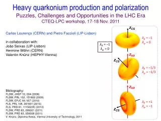
Frames and parameters z Collins-Soperaxis (CS): ≈ dir. of colliding partons Helicity axis (HX): dir. of quarkonium momentum quarkonium rest frame θ ℓ + production plane φ y x λθ = +1 λφ = λθφ = 0 λθ = +1 : “transverse” (= photon-like) pol. Jz= ± 1 λθ = –1 λφ = λθφ = 0 λθ = 1 : “longitudinal”pol. Jz= 0 z′ z CS HX for mid rap. / high pT HX CS 90º x x′ y y′
Frames and parameters z Collins-Soperaxis (CS): ≈ dir. of colliding partons Helicity axis (HX): dir. of quarkonium momentum quarkonium rest frame θ ℓ + production plane φ y x λθ = +1 λφ = λθφ = 0 λθ = +1 : “transverse” (= photon-like) pol. Jz= ± 1 λθ = –1 λφ = λθφ = 0 λθ = 1 : “longitudinal”pol. Jz= 0 z′ z CS HX for mid rap. / high pT HX CS 90º x x′ y y′
The azimuthal anisotropy is not a detail Case 2: natural longitudinal polarization, observation frame to the natural one Case 1: natural transverse polarization z z Jx = 0 x x Jz= ± 1 λθ = +1 λφ = 0 λθ = +1 λφ = 1 y y • Two very different physical cases • Indistinguishable if λφ is not measured (integration over φ)
Frame-independent polarization The shape of the distribution is obviously frame-invariant. → it can be characterized by a frame-independent parameter, e.g. z λθ = –1 λφ = 0 λθ = +1 λφ = 0 λθ = –1/3 λφ = –1/3 λθ = +1/5 λφ = +1/5 λθ = +1 λφ = –1 λθ = –1/3 λφ = +1/3 FLSW, PRL 105, 061601; PRD 82, 096002; PRD 83, 056008
J=1 states are intrinsically polarized Singleelementary subprocess: There is no combination ofa0, a+1and a-1such thatλθ = λφ = λθφ = 0 The angular distribution is never intrinsically isotropic Only a “fortunate” mixture of subprocesses (or randomization effects) can lead to a cancellation of allthreeobservedanisotropy parameters To measure zero polarization would be(in fact, is) an exceptionally interesting result...
Positivity constraints for dilepton distributions P. F., C.L., J.S., Phys. Rev. D 83, 056008 (2011) • General and frame-independent constraints on the anisotropy parameters of vector particle decays JyV = 0 λφ JxV = ±V ~ λ = +1 Jz V = 0 JzV = ±V ~ λ = –1 JyV = ±V JxV = 0 λθ λθφ λθφ physical domain λθ λφ
What polarization axis? 1) helicity conservation (at the production vertex) → J =1 states produced in fermion-antifermion annihilations (q-q or e+e–) at Born level have transverse polarization along the relative direction of the colliding fermions (Collins-Soperaxis) 1 . 5 ( ) Drell-Yan is a paradigmatic case but not the only one Drell-Yan 1 . 0 (2S+3S) λθ 0 . 5 z(HX) E866 (p-Cu) Collins-Soper frame 0 . 0 90° high pT z(CS) - 0 . 5 0 1 2 pT[GeV/c] c g 2) NRQCD → at very large pT , quarkonium produced from the fragmentation of an on-shell gluon, inheriting its natural spin alignment c g J/ψ NRQCD λθ g g CDF → large, transverse polarization along the QQ (=gluon) momentum(helicityaxis) pT [GeV/c]
Example: Drell-Yan, Z and W polarization • always fully transverse polarization • but with respect to a subprocess-dependent quantization axis V = *, Z, W _ Due to helicity conservation at the q-q-V (q-q*-V)vertex, Jz = ± 1 along the q-q (q-q*) scattering direction z _ z q z = relative dir. of incoming q and qbar (Collins-Soper) _ _ V q q ~ ~ ~ ~ λ = +1 λ = +1 λ = +1 λ = +1 V q z = dir. of one incoming quark (Gottfried-Jackson) q V q* q* g QCD corrections z = dir. of outgoing q (cms-helicity) q V q* g q the Lam-Tung relation simply derives from rotational invariance + helicity conservation! Note:
Basic meaning of the frame-invariant quantities Let us suppose that, in the collected events, n different elementary subprocesses yield angular momentum states of the kind (wrt a given quantization axis), each one with probability . The rotational properties of J=1 angular momentum states imply that The quantity is therefore frame-independent. It can be shown to be equal to In other words, there always exists a calculable frame-invariant relation of the form the combinations are independent of the choice of the quantization axis
Simple derivation of the Lam-Tung relation Another consequence of rotational properties of angular momentum eigenstates: for each state there exists a quantization axis wrt which → dileptons produced in each single elementary subprocess have a distribution of the type wrt its specific “ ” axis. DY: q q q * * * * q* q* q* _ q q _ Due to helicity conservation at the q-q-* (q-q*-*)vertex, along the q-q (q-q*) scattering direction _ →for each diagram sum independent of spin alignment directions! Lam-Tung identity →
Essence of the LT relation The existence (and frame-independence) of the LT relation is the kinematic consequence of the rotational properties of J = 1 angular momentum eigenstates Its form derives from the dynamical input that all contributing processes produce a transversely polarized (Jz = ±1) state (wrt whatever axis) More generally: • Corrections to the Lam-Tung relation (parton-kT, higher-twist effects) should continue to yield invariant relations.In the literature, deviations are often searched in the form • But this is not a frame-independent relation. Rather, corrections should be searched in the invariant form • For any superposition of processes, concerning anyJ = 1 particle (even in parity-violating cases: W, Z), we can always calculate a frame-invariant relation analogous to the LT relation.
Reference frames are not all equally good Especially relevant when the production mechanisms and the resulting polarization are a priori unknown (quarkonium, but also newly discovered particles) Gedankenscenario: how would different experiments observe a Drell-Yan-like decay distribution 1 + cos2θ in the Collins-Soper frame with an arbitrary choice of the reference frame? Consider decay. For simplicity: each experiment has a flat acceptance in its nominal rapidity range:
The lucky frame choice (CS in this case)
Less lucky choice (HX in this case) +1/3 λθ = +0.65 λθ = 0.10 1/3 artificial dependence on pT and on the specific acceptance • look for possible “optimal” frame • avoid kinematic integrations
Advantages of “frame-invariant” measurements Gedankenscenario: Consider this (purely hypothetic) mixture of subprocesses for production: 60% of the events have a natural transverse polarization in the CS frame 40% of the events have a natural transverse polarization in the HX frame As before:
Frame choice 1 All experiments choose the CS frame
Frame choice 2 All experiments choose the HX frame No “optimal” frame in this case...
Any frame choice The experiments measure an invariant quantity, for example ~ ~ Using λ we measure an “intrinsic quality” of the polarization (always transverse and kinematics-independent, in this case) Frame-invariant quantities • are immune to “extrinsic” kinematic dependencies • minimize the acceptance-dependence of the measurement • facilitate the comparison between experiments, and between data and theory • can be used as a cross-check: is the measured λ identical in different frames?(not trivial: spurious anisotropies induced by the detector do not have the qualities of a J = 1 decay distribution) λθ + 3 λφ λ = 1 λφ ~ [PRD 81, 111502(R) (2010), EPJC 69, 657 (2010)]
Some remarks on methodology • Measurements are challenging • A typical collider experiment imposes pT cuts on the single muons;this creates zero-acceptance domains in decay distributions from “low” masses: helicity Collins-Soper φHX φCS Toy MC with pT(μ) > 3 GeV/c (both muons) Reconstructed unpolarized(1S) pT() > 10 GeV/c, |y()| < 1 cosθHX cosθCS • This spurious “polarization” must be accurately taken into account. • Large holes strongly reduce the precision in the extracted parameters • In the analyses we must avoid simplifications that make the present results sometimes difficult to be interpreted: • only λθmeasured, azimuthal dependence ignored • one polarization frame “arbitrarily” chosen a priori • no rapidity dependence
Some remarks on methodology Definition of the PPD dimuonefficiency as functionof muon momenta general shapeofthe angular distribution uniform integral ofW εover cosθ, φ (withdistributionsofremainingleptondegreesoffreedomtakenfrom data)
Some remarks on methodology Extraction of results
30 Quarkonium polarization: a “puzzle” • J/𝜓: Measurements at Tevatron , LHC (ALICE) _ J/ψ, pp √s = 1.96 TeV CDF Run I CDF Run II |y| < 0.4 CDF II vs CDF I → not known what caused the change |y| < 0.6 Helicity frame PRL 85, 2886 (2000) PRL 99, 132001 (2007) J/ψ, pp √s = 7 TeV ALICE 2.5 < y < 4, 2 < pT < 8 GeV/c PRL 108, 082001 (2012)
31 Quarkonium polarization: a “puzzle” • J/𝜓: HERA-B J/ψ, p-Cu and p-W √s = 41.6 GeV EPJ C60 517 (2009)
32 Quarkonium polarization: a “puzzle” • J/𝜓: Other fixed target experiments (E537-fixed target A=(Cu, W, Be)) PRD 48, 5076 (1993)
33 Quarkonium polarization: a “puzzle” • J/𝜓: Other fixed target experiments Chicago-Iowa-Princeton Coll. PRL 58, 2523 (1987)
Quarkonium polarization: a “puzzle” 34 • 𝜰(nS): Measurements at Tevatron (2002-2012) _ (1S), pp √s = 1.96 TeV |y| < 0.4 √s = 1.8 TeV (2002) |y| < 0.6 |y| < 1.8 PRL 88, 161802 (2002) PRL 108, 151802 (2012) PRL 101, 182004 (2008) CDF vs D0 :Can a strong rapidity dependence justify the discrepancy?
Quarkonium polarization: a “puzzle” 35 • 𝜰(nS): Measurements at Tevatron (2002-2012) _ (1S), pp √s = 1.96 TeV
36 Quarkonium polarization: a “puzzle” • 𝜰(nS): Measurements at LHC (CMS) (nS), pp √s = 7 TeV |y| < 0.6 0.6<|y| < 1.2 arXiv:1209.2922[hep-ex] to appear in PRL Comparison with CDF results
37 Quarkonium polarization: a “puzzle” • 𝜰(nS): Measurements at LHC (CMS) (nS), pp √s = 7 TeV |y| < 0.6 0.6<|y| < 1.2 arXiv:1209.2922[hep-ex] to appear in PRL Comparison with CDF results
38 Quarkonium polarization: a “puzzle” • 𝜰(nS): Measurements at LHC (CMS) (nS), pp √s = 7 TeV
39 Quarkonium polarization: a “puzzle” • 𝜰(nS): Mesurements at LHC (CMS) (nS), pp √s = 7 TeV
40 Quarkonium polarization: a “puzzle” • 𝜰(nS): E866/NuSea Most reasonable explanation is that most 𝜰(1S) come from b and have very different polarization (nS), p-Cu √s = 38.8 GeV pT> 1.8 GeV/c
Direct vs. prompt J/ψ The direct-J/ψ polarization (cleanest theory prediction) can be derived from the prompt-J/ψ polarization measurement of CDF knowing • the χc-to-J/ψ feed-down fractions • the χc polarizations CDF data R(χc1)+R(χc2) = 30 ± 6 % R(χc2)/R(χc1) = 40 ± 2 % CDF prompt J/ψ CDF prompt J/ψ extrapolated direct J/ψ CSM direct J/ψ extrapolated direct J/ψ taking central values using the valuesR(χc1)+R(χc2) = 42 % (+2σ)R(χc2)/R(χc1) = 38 % (-1σ)the CSM prediction of direct-J/ψ polarization agrees very well with the CDF data in the scenario h(χc1) = 0 and h(χc2) = ±2 possible combinations of pure χc helicity states helicity frame helicity frame Direct-J/ψ: 𝜆 = -0.6 From c: 𝜆 = +1 χc measurements are crucial !
A lot of measurements to do... • Measurement of c0(1P), c1(1P) and c2(1P) production cross sections • Measurement of b (1P), b(2P) and b(3P) production cross sections; • Measurement of the relative production yields of J = 1 and J = 2 b states • Measurement of the c1 (1P) and c2(1P) polarizations versus pT and rapidity • Measurement of the b (1P) and b (2P) polarizations • …
J/ψpolarization as a signal of colour deconfinement? ≈ 0.7 ≈ 0.7 λθ HX frame CS frame • J/ψ significantly polarized (high pT) • feeddown from χc states (≈ 30%) smears the polarizations Starting “pp” scenario: J/ψ cocktail: NRQCD Si λθ Sequential suppression ≈ 30% from χc decays ≈ 70% direct J/ψ + ψ’ decays pT [GeV/c] Recombination ? e • As the χc (and ψ’) mesons get dissolved by the QGP, λθ should change to its direct value
J/ψ polarization as a signal of sequential suppression? P. Faccioli, JS, PRD 85, 074005 (2012) • CMS data: • up to 80% of J/ψ’s disappear from pp to Pb-Pb • more than 50%( fraction of J/ψ’s from ψ’ andχc)disappear from peripheral to central collisions CMS PAS HIN-10-006 • sequential suppression gedankenscenario:in central events ψ’ andχcare fully suppressedand all J/ψ’s are direct ~ > It may be impossible to test this directly: measuring the χc yield (reconstructing χc radiative decays) in PbPb collisions is prohibitively difficult due to the huge number of photons However, a change of prompt-J/ψ polarization must occur from pp to central Pb-Pb! prompt J/ψ polarization in pp χc-to-J/ψ fractions in pp χc polarizations in pp prompt J/ψ polarization in PbPb Reasonable sequence of measurements: χc suppression in PbPb!
J/ψ polarization as a signal of sequential suppression? Example scenario: CDF prompt J/ψ Extrapolated* direct J/ψ CSM direct J/ψ prompt-J/ψ polarization in pp: λθ – 0.15 direct-J/ψ polarization: λθ – 0.6 helicity frame (assumed to be the same in pp and PbPb) * R(χc1)+R(χc2) = 42 % R(χc2)/R(χc1) = 38 %h(χc1) = 0 h(χc2) = ±2
J/ψ polarization as a signal of sequential suppression? “prompt” λθ If we measure a change in prompt polarization like this... “direct” ... we are observing the disappearance of the χc relative to the J/ψ R(χc) in PbPb R(χc) in pp • Simplifying assumptions: • direct-J/ψ polarization is the same in pp and PbPb • normal nuclear effects affect J/ψ and χcin similar ways • χc1 and χc2 are equally suppressed in PbPb
J/ψ polarization as a signal of sequential suppression? When will we be sensitive to an effect like this? pT(μ) > 3 GeV/c, 6.5 < pT < 30 GeV/c, 0 < |y| < 2.4 CMS-like toy MC with prompt-J/ψ polarization as observed in pp (and peripheral PbPb) prompt-J/ψ polarization as observed in central PbPb efficiency-corrected |cosθHX| distribution precise results in pp very soon ~20k evts ~20k evts In this scenario, the χc disappearance is measurable at ~5σ level with ~20k J/ψ’s in central Pb-Pb collisions
J/ψ polarization as a signal of sequential suppression? When will we be sensitive to an effect like this? CMS-like toy MC
Summary • The new quarkonium polarization measurements have many improvements with respect to previous analysesWill we manage to solve an old puzzle? • General advice: do not throw away physical information!(azimuthal-angle distribution, rapiditydependence, ...) • A new method based on rotation-invariant observablesgives several advantages in the measurement of decay distributions and in the use of polarizationinformation • Charmonium polarization can be used to probe QGP formation