Understanding Functions and Files in MATLAB: Getting Help and Common Operations
1.04k likes | 1.32k Vues
This PowerPoint presentation accompanies Chapter 3 of "Introduction to MATLAB for Engineers, Third Edition," focusing on functions and file operations in MATLAB. It covers the use of the `lookfor` command to find relevant functions, common mathematical functions, operations with complex numbers, and array operations. The material emphasizes keyboard syntax for function arguments, common mistakes in function usage, trigonometric functions in radian mode, and the creation of user-defined functions. This content is essential for mastering MATLAB for engineering applications.

Understanding Functions and Files in MATLAB: Getting Help and Common Operations
E N D
Presentation Transcript
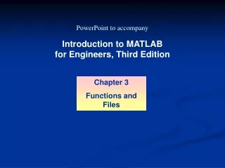
PowerPoint to accompany Introduction to MATLAB for Engineers, Third Edition Chapter 3 Functions and Files
3-2 Getting Help for Functions You can use the lookfor command to find functions that are relevant to your application. For example, type lookfor imaginary to get a list of the functions that deal with imaginary numbers. You will see listed: imag Complex imaginary part i Imaginary unit j Imaginary unit More? See pages 113-114.
Common mathematical functions: Table 3.1–1, page 114 3-3 Exponential; e x Square root; x Natural logarithm; ln x Common (base 10) logarithm; log x = log10x (continued…) Exponential exp(x) sqrt(x) Logarithmic log(x) log10(x)
Complex abs(x) angle(x) conj(x) imag(x) real(x) Absolute value. Angle of a complex number. Complex conjugate. Imaginary part of a complex number. Real part of a complex number. (continued…) Some common mathematical functions (continued) 3-4
Numeric ceil(x) fix(x) floor(x) round(x) sign(x) Round to nearest integer toward ∞. Round to nearest integer toward zero. Round to nearest integer toward -∞. Round toward nearest integer. Signum function: +1 if x >0; 0 if x = 0; -1 if x <0. Some common mathematical functions (continued) 3-5
The rectangular and polar representations of the complex number a + ib. 3-6
3-7 Operations with Complex Numbers >>x = -3 + 4i; >>y = 6 - 8i; >>mag_x = abs(x) mag_x = 5.0000 >>mag_y = abs(y) mag_y = 10.0000 >>mag_product = abs(x*y) 50.0000 (continued …)
3-8 Operations with Complex Numbers (continued) >>angle_x = angle(x) angle_x = 2.2143 >>angle_y = angle(y) angle_y = -0.9273 >>sum_angles = angle_x + angle_y sum_angles = 1.2870 >>angle_product = angle(x*y) angle_product = 1.2870
3-9 Operations on Arrays MATLAB will treat a variable as an array automatically. For example, to compute the square roots of 5, 7, and 15, type >>x = [5,7,15]; >>y = sqrt(x) y = 2.2361 2.6358 3.8730
3-10 Expressing Function Arguments We can write sin 2 in text, but MATLAB requires parentheses surrounding the 2 (which is called the function argument or parameter). Thus to evaluate sin 2 in MATLAB, we type sin(2). The MATLAB function name must be followed by a pair of parentheses that surround the argument. To express in text the sine of the second element of the array x, we would type sin[x(2)]. However, in MATLAB you cannot use square brackets or braces in this way, and you must type sin(x(2)). (continued …)
3-11 Expressing Function Arguments (continued) To evaluate sin(x 2 + 5), you type sin(x.^2 + 5). To evaluate sin(x+1), you type sin(sqrt(x)+1). Using a function as an argument of another function is called function composition. Be sure to check the order of precedence and the number and placement of parentheses when typing such expressions. Every left-facing parenthesis requires a right-facing mate. However, this condition does not guarantee that the expression is correct!
3-12 Expressing Function Arguments (continued) Another common mistake involves expressions like sin2x, which means (sin x)2. In MATLAB we write this expression as (sin(x))^2, not as sin^2(x),sin^2x, sin(x^2), or sin(x)^2!
3-13 Expressing Function Arguments (continued) The MATLAB trigonometric functions operate in radian mode. Thus sin(5) computes the sine of 5 rad, not the sine of 5°. To convert between degrees and radians, use the relation qradians = (p /180)qdegrees.
Trigonometric functions: Table 3.1–2, page 116 3-14 Cosine; cos x. Cotangent; cot x. Cosecant; csc x. Secant; sec x. Sine; sin x. Tangent; tan x. cos(x) cot(x) csc(x) sec(x) sin(x) tan(x)
acos(x) acot(x) acsc(x) asec(x) asin(x) atan(x) atan2(y,x) Inverse cosine; arccos x. Inverse cotangent; arccot x. Inverse cosecant; arccsc x. Inverse secant; arcsec x. Inverse sine; arcsin x . Inverse tangent; arctan x . Four-quadrant inverse tangent. Inverse Trigonometric functions: Table 3.1–2 3-15
Hyperbolic functions: Table 3.1–3, page 119 3-16 Hyperbolic cosine Hyperbolic cotangent. Hyperbolic cosecant Hyperbolic secant Hyperbolic sine Hyperbolic tangent cosh(x) coth(x) csch(x) sech(x) sinh(x) tanh(x)
acosh(x) acoth(x) acsch(x) asech(x) asinh(x) atanh(x) Inverse hyperbolic cosine Inverse hyperbolic cotangent Inverse hyperbolic cosecant Inverse hyperbolic secant Inverse hyperbolic sine Inverse hyperbolic tangent; Inverse Hyperbolic functions: Table 3.1–3 3-17
3-18 User-Defined Functions The first line in a function file must begin with a function definition line that has a list of inputs and outputs. This line distinguishes a function M-file from a script M-file. Its syntax is as follows: function [output variables] = name(input variables) Note that the output variables are enclosed in square brackets, while the input variables must be enclosed with parentheses. The function name (here, name) should be the same as the file name in which it is saved (with the .m extension). More? See pages 119-123.
3-19 User-Defined Functions: Example function z = fun(x,y) u = 3*x; z = u + 6*y.^2; Note the use of a semicolon at the end of the lines. This prevents the values of u and z from being displayed. Note also the use of the array exponentiation operator (.^). This enables the function to accept y as an array. (continued …)
3-20 User-Defined Functions: Example (continued) Call this function with its output argument: >>z = fun(3,7) z = 303 The function uses x = 3 and y = 7 to compute z. (continued …)
3-21 User-Defined Functions: Example (continued) Call this function without its output argument and try to access its value. You will see an error message. >>fun(3,7) ans = 303 >>z ??? Undefined function or variable ’z’. (continued …)
3-22 User-Defined Functions: Example (continued) Assign the output argument to another variable: >>q = fun(3,7) q = 303 You can suppress the output by putting a semicolon after the function call. For example, if you type q = fun(3,7); the value of q will be computed but not displayed (because of the semicolon).
3-23 Local Variables: The variables x and y are local to the function fun, so unless you pass their values by naming them x and y, their values will not be available in the workspace outside the function. The variable u is also local to the function. For example, >>x = 3;y = 7; >>q = fun(x,y); >>x x = 3 >>y y = 7 >>u ??? Undefined function or variable ’u’.
3-24 Only the order of the arguments is important, not the names of the arguments: >>x = 7;y = 3; >>z = fun(y,x) z = 303 The second line is equivalent to z = fun(3,7).
3-25 You can use arrays as input arguments: >>r = fun(2:4,7:9) r = 300 393 498
3-26 A function may have more than one output. These are enclosed in square brackets. For example, the function circle computes the area A and circumference C of a circle, given its radius as an input argument. function [A, C] = circle(r) A = pi*r.^2; C = 2*pi*r;
The function is called as follows, if the radius is 4. >>[A, C] = circle(4) A = 50.2655 C = 25.1327 3-27
A function may have no input arguments and no output list. For example, the function show_date clears all variables, clears the screen, computes and stores the date in the variable today, and then displays the value of today. function show_date clear clc today = date 3-28
3-29 Examples of Function Definition Lines • One input, one output: function [area_square] = square(side) 2. Brackets are optional for one input, one output: function area_square = square(side) 3. Two inputs, one output: function [volume_box] = box(height,width,length) 4. One input, two outputs: function [area_circle,circumf] = circle(radius) 5. No named output: function sqplot(side)
Function Example function [dist,vel] = drop(g,vO,t); % Computes the distance travelled and the % velocity of a dropped object, % as functions of g, % the initial velocity vO, and % the time t. vel = g*t + vO; dist = 0.5*g*t.^2 + vO*t; (continued …) 3-30
Function Example (continued) 1. The variable names used in the function definition may, but need not, be used when the function is called: >>a = 32.2; >>initial_speed = 10; >>time = 5; >>[feet_dropped,speed] = . . . drop(a,initial_speed,time) (continued …) 3-31
Function Example (continued) 2. The input variables need not be assigned values outside the function prior to the function call: [feet_dropped,speed] = drop(32.2,10,5) 3. The inputs and outputs may be arrays: [feet_dropped,speed]=drop(32.2,10,0:1:5) This function call produces the arrays feet_dropped and speed, each with six values corresponding to the six values of time in the array time. 3-32
Local Variables The names of the input variables given in the function definition line are local to that function. This means that other variable names can be used when you call the function. All variables inside a function are erased after the function finishes executing, except when the same variable names appear in the output variable list used in the function call. 3-33
Global Variables The global command declares certain variables global, and therefore their values are available to the basic workspace and to other functions that declare these variables global. The syntax to declare the variables a, x, and q is globala x q Any assignment to those variables, in any function or in the base workspace, is available to all the other functions declaring them global. More? See pages 124. 3-34
3-35 Function Handles You can create a function handle to any function by using the at sign, @, before the function name. You can then use the handle to reference the function. To create a handle to the function y =x + 2e-x-3, define the following function file: function y = f1(x) y = x + 2*exp(-x) - 3; You can pass the function as an argument to another function. For example, we can plot the functionover 0 £x £ 6 as follows: >>plot(0:0.01:6,@f1)
Finding Zeros of a Function You can use the fzero function to find the zero of a function of a single variable, which is denoted by x. One form of its syntax is fzero(@function, x0) where @function is the function handle for the function function, and x0 is a user-supplied guess for the zero. The fzero function returns a value of x that is near x0. It identifies only points where the function crosses the x-axis, not points where the function just touches the axis. For example, fzero(@cos,2) returns the value 1.5708. 3-36
Using fzero with User-Defined Functions To use the fzero function to find the zeros of more complicated functions, it is more convenient to define the function in a function file. For example, if y =x + 2e-x-3, define the following function file: function y = f1(x) y = x + 2*exp(-x) - 3; (continued …) 3-37
Plot of the function y =x + 2e-x- 3. Figure 3.2–1, page 125 There is a zero near x = -0.5 and one near x = 3. 3-38 (continued …)
Example (continued) To find a more precise value of the zero near x = -0.5, type >>x = fzero(@f1,-0.5) The answer is x = -0.5881. More? See pages 125-126. 3-39
Finding the Minimum of a Function The fminbnd function finds the minimum of a function of a single variable, which is denoted by x. One form of its syntax is fminbnd(@function, x1, x2) where @function is the function handle for the function. The fminbnd function returns a value of x that minimizes the function in the interval x1 ≤ x ≤ x2. For example, fminbnd(@cos,0,4) returns the value 3.1416. 3-40
When using fminbnd it is more convenient to define the function in a function file. For example, if y = 1 -xe -x, define the following function file: function y = f2(x) y = 1-x.*exp(-x); To find the value of x that gives a minimum of y for 0 £x £ 5, type >>x = fminbnd(@f2,0,5) The answer is x = 1. To find the minimum value of y, type y = f2(x). The result is y = 0.6321. 3-41
A function can have one or more local minima and a global minimum. If the specified range of the independent variable does not enclose the global minimum, fminbnd will not find the global minimum. fminbnd will find a minimum that occurs on a boundary. 3-42
Plot of the function y = 0.025x 5- 0.0625x 4- 0.333x 3+x 2. Figure 3.2–2 This function has one local and one global minimum. On the interval [1, 4] the minimum is at the boundary, x = 1. 3-43
To find the minimum of a function of more than one variable, use the fminsearch function. One form of its syntax is fminsearch(@function, x0) where @function is the function handle of the function in question. The vector x0 is a guess that must be supplied by the user. 3-44
To minimize the function f = xe-x2- y2, we first define it in an M-file, using the vector x whose elements are x(1) = x and x(2) = y. function f = f4(x) f = x(1).*exp(-x(1).^2-x(2).^2); Suppose we guess that the minimum is near x = y = 0. The session is >>fminsearch(@f4,[0,0]) ans = -0.7071 0.000 Thus the minimum occurs at x = -0.7071, y = 0. 3-45
Methods for Calling Functions There are four ways to invoke, or “call,” a function into action. These are: • As a character string identifying the appropriate function M-file, 2. As a function handle, 3. As an “inline” function object, or 4. As a string expression. Examples of these ways follow for the fzero function used with the user-defined function fun1, which computes y = x2- 4. (continued …) 3-46
Methods for Calling Functions (continued) 1. As a character string identifying the appropriate function M-file, which is function y = fun1(x) y = x.^2-4; The function may be called as follows, to compute the zero over the range 0 £x £ 3: >>[x, value] = fzero(’fun1’,[0, 3]) (continued …) 3-47
Methods for Calling Functions (continued) 2. As a function handle to an existing function M-file: >>[x, value] = fzero(@fun1,[0, 3]) 3. As an “inline” function object: >>fun1 = ’x.^2-4’; >>fun_inline = inline(fun1); >>[x, value] = fzero(fun_inline,[0, 3]) (continued …) 3-48
Methods for Calling Functions (continued) 4. As a string expression: >>fun1 = ’x.^2-4’; >>[x, value] = fzero(fun1,[0, 3]) or as >>[x, value] = fzero(’x.^2-4’,[0, 3]) (continued …) 3-49
Methods for Calling Functions (continued) The function handle method (method 2) is the fastest method, followed by method 1. In addition to speed improvement, another advantage of using a function handle is that it provides access to subfunctions, which are normally not visible outside of their defining M-file. More? See pages 130-131. 3-50