Introduction to Optimization
Introduction to Optimization. Outline. Conventional design methodology What is optimization? Unconstrained minimization Constrained minimization Global-Local Approaches Multi-Objective Optimization Optimization software Structural optimization Surrogate optimization ( Metamodeling )


Introduction to Optimization
E N D
Presentation Transcript
Outline • Conventional design methodology • What is optimization? • Unconstrained minimization • Constrained minimization • Global-Local Approaches • Multi-Objective Optimization • Optimization software • Structural optimization • Surrogate optimization (Metamodeling) • Summary
Conventional Design Method Initial design Analyze the system Is design satisfactory ? No Change design based on experience
Conventional Design Method • Depends on the designer’s intuition, experience, and skill • Is a trial-and-error method • Is not easy to apply to a complex system • Does not always lead to the best possible design • Is a qualitative design
N w t N What is optimization? • Optimization discipline deals with finding the maxima and minima of functions subject to some constraints. Typical problem formulation: Given p………………..parameters of the problem Find d………………..the design variables of the problem Min f(d,p)…………...objective function Subject to g(d,p)≤0………..inequality constraints h(d,p)=0………..equality constraints dL≤ d ≤ dU………lower and upper bounds • Example: Point stress design for minimum weight Given w, N Find t Min t (i.e., weight) S.t. σ – σcrit = N/(w t) – σY ≤0 tL≤ t ≤ tU
Definitions Design variables (d): A design variable is a specification that is controllable by the designer (eg., thickness, material, etc.) and are often bounded by maximum and minimum values. Sometimes these bounds can be treated as constraints. Constraints (g, h): A constraint is a condition that must be satisfied for the design to be feasible. Examples include physical laws, constraints can reflect resource limitations, user requirements, or bounds on the validity of the analysis models. Constraints can be used explicitly by the solution algorithm or can be incorporated into the objective using Lagrange multipliers. Objectives (f): An objective is a numerical value or function that is to be maximized or minimized. For example, a designer may wish to maximize profit or minimize weight. Many solution methods work only with single objectives. When using these methods, the designer normally weights the various objectives and sums them to form a single objective. Other methods allow multi-objective optimization, such as the calculation of a Pareto front. Models: The designer must also choose models to relate the constraints and the objectives to the design variables. They may include finite element analysis, reduced order metamodels, etc. Reliability: the probability of a component to perform its required functions under stated conditions for a specified period of time
f(x) Unconstrained minimization (1-D) • Find the minimum of a function • Derivatives • at local max or local min, f’(x)=0 • f”(x) > 0 if local min • f”(x) < 0 if local max • f”(x) = 0 if saddlepoint
Hessian Unconstrained minimization (n-D) • Optimality conditions • Necessary condition f = 0 • Sufficient condition H is positive definite (H: Hessian matrix; matrix of 2nd derivatives) • Gradient based methods Steepest descent method Conjugate gradient method Newton and quasi-Newton methods (best known is BFGS)
Optimization Methods • Commercial Tools • BOSS quattro (SAMTECH) • FEMtools Optimization (Dynamic Design Solutions) • HEEDS (Red Cedar Technology) • HyperWorksHyperStudy (Altair Engineering) • IOSO (Sigma Technology) • Isight (DassaultSystèmesSimulia) • LS-OPT (Livermore Software Technology Corporation) • modeFRONTIER (Esteco) • ModelCenter (PhoenixIntegration) • Optimus (Noesis Solutions) • OptiY (OptiYe.K.) • VisualDOC (Vanderplaats Research and Development) • SmartDO (FEA-Opt Technology) • MATLAB • Unconstrained: BFGS(fminunc), Simplex(fminsearch) • Constrained: SQP(fmincon)_ • Visual DOC • Unconstrained: BFGS, Fletcher-Reeves • Constrained: SLP, SQP, Method of feasible directions • Gradient-based methods • Adjoint equation • Newton’s method • Steepest descent • Conjugate gradient • Sequential quadratic programming • Gradient-free methods • Hooke-Jeeves pattern search • Nelder-Mead method • Population-based methods • Genetic algorithm • Memetic algorithm • Particle swarm optimization • Ant colony • Harmony search • Other methods • Random search • Grid search • Simulated annealing • Direct search • IOSO(Indirect Optimization based on Self-Organization)
Evolutionary (Non-gradient) algorithms • Initialization:initialize population of solutions (physical & search parameter sets) • Reproduction:mutate and/or recombine solutions to produce next generation • Evaluate Fitness:compute objectives & fitness (DEA efficiencies) of new generation • Selection: Select which solutions survive to next generation and possibly reproduce • Termination:decide when to stop evolution
Termination - stall criteria • Specify a maximum number of generations past which the system cannot evolve • Retain best solutions in “elite” population; these are kept separate from solutions in “evolving” • population and consist of best solutions obtained regardless of age • Keep running averages of each objective of the solutions in elite population over a window of, • say, 50 generations • When running average stops changing by more • than some tolerance, terminate evolution
Characteristics of evolutionary algorithms • Very flexible; there are very many implementations of evolutionary algorithms • Choice of implementation is often dictated by the representation of the solution to a particular problem • Successful over wide range of difficult problems in nonlinearoptimization • Constraints problematic – multiple objective methods often employed • Require many evaluations of objective functions but these are inherently parallel
Gradient-/Population-Based Methods • Gradient-based methods are commonly used, but may suffer from… • Dependence on the starting point • Convergence to local optima • Population-based methods are high likely to find the global optimum, but are computation- ally more expensive
quadratic linear Guaranteed optimum solution Constrained minimization • Gradient projection methods • Find good direction tangent to active constraints • Move a distance and then restore to constraint boundaries • Method of feasible directions • A compromise between objective reduction and constraint avoidance • Penalty function methods • Sequential approximation methods • Sequential quadratic programming Iteratively approximate as QP
Global-Local Optimization Approaches • Global Methods • Population based methods • Genetic algorithm • Memetic algorithm • Particle swarm optimization • Ant colony • Harmony search global local parameter space Local Methods • Gradient Based • Newton’s method (unconstrained) • Steepest descent (unconstrained) • Conjugate gradient (unconstrained) Sequential Unconstrained Minimization Techniques (SUMT) (constrained) • Sequential linear programming (constrained) • Sequential quadratic programming (constrained) • Modified Method of Feasible Directions (constrained) • Evolutionary (no history) Simplex Method (SM) Genetic Algorithms (GA) Differential Evolution
Constrained Optimization • Identify : • Design variables (X) • Objective functions to be minimized (F) • Constraints that must be satisfied (g) Starting point Initial design Analysis Analyze the system Optimizer Convergence criteria ? Converge ? Updated No No Change design using Optimization technique
Courtesy of Venkataraman and Haftka* (2004) Need for a metamodel • Venkataraman and Haftka* (2004) reported that analysis models of acceptable accuracy have required at least six to eight hours of computer time (an overnight run) throughout the last thirty years, even though computer processing power, memory and storage space have increased drastically. • Because fidelity and complexity of analysis models required by designers increased. • There has been a growing interest in replacing these slow, expensive and mostly noisy simulations with smooth approximate models that produce fast results. • These approximate models (functional relationships between input and output variables) are referred to as metamodels or surrogate models. * Venkataraman S, and Haftka RT (2004). “Structural optimization complexity: what has Moore’s law done for us?” Structural and Multidisciplinary Optimization, 28: 375–387.
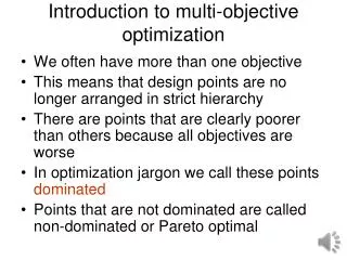
Multiple objective optimization A set of decision variables that forms a feasible solution to a multiple objective optimization problem is Pareto dominant;if there exists no other such set that could improve one decision variable without making at least one other decision variable worse. Vilfredo Pareto
Convergence of pareto frontier One dimensional objective space • It is relatively simple to determine an optimal solution for single objective methods (solution with the lowest error function) • However, for multiple objectives, we must evaluate solutions on a “Pareto frontier” • A solution lies on the Pareto frontier when any further changes to the parameters result in one or more objectives improving with the other objective(s) suffering as a result • Once a set of solutions have converged to the Pareto frontier, further testing is required in order to determine which candidate force field is optimal for the problems of interest • Be aware that searches with a limited number of parameters might “cram” a lot of important physics into a few parameters Error function Iteration Two dimensional objective space converged Pareto surface
Model Calibration Optimization Find parameters: λ1,…,λd That reproduce properties: pkλ1,…,λd ( ) Via some objective fxn: g( λ1,…,λd ) = Σwk (pk − p*k )2 But not a downhill stroll: - Many-dimensional - Expensive function evaluation - No analytical gradients - Noisy properties
Define optimization problem Min f(x1, x2…xn) s.t. g(x) ≤ 0 h(x) = 0 f g h x1 x2 … xn Metamodel Evaluatef(x), g(x), h(x) • Refine design space • Add more data points No Identify most and least important variables using GSA Validation? Yes Perform optimiza- tion Stop (not necessary but advisable) Metamodeling based optimization (MBO)
Surrogate Modeling (Metamodels or Response Surface Methodology) A method for constructing global approximations to system behavior based on results calculated at various design variable sets in the design space. Linear Elliptic Quadratic Surface fitting to calculate coefficients,
Procedure of Surrogate Design Optimization Statistical process to obtain optimum design variable set to minimize (or maximize) objective functions which satisfying constraints Identify : Design variables (important controllable parameters to describe a system) Objective functions (design goals or criteria) to be minimized or maximized Constraints (design limitations or restrictions) that must be satisfied Metamodeling (Surrogate Modeling) Interpolation Methods Radial Basis Functions Neural Networks Regression Methods Polynomial Response Surface (PRS) Support Vector Regression (SVR) Multivariate adaptive regression splines (reg) Gaussian Process (GP) Hybrids Krigingmethod (int+reg) Ensemble (all methods) Optimization - Find an optimal design variable set -Bayesian -Optimization algorithms (evolutionary-not gradient based) - FDM, SUMT, LP, GA Multi-objective function formulations - UFF, GCF, GTA - Multi-level approach Multi-start local optimization DOE methods - Select design points that must be analyzed Central composite design Factorial design Plackett-Burman Koshal design Latin hypercube sampling D-optimal design Taguchi's orthogonal array Monte Carlo method Analysis - Analyze system using computational methods ABAQUS FEA LS-Dyna FEA Pamcrash FEA MegaMas DD LAMMPS MD VASP
Surrogate-Based Optimization (Metamodeling or Response Surface Methods) DOE Selected Analysis Metamodel Approximation Benefit: quicker answers Issue: less accuracy (maybe) Objective – Develop metamodels as low-cost surrogates for expensive high-fidelity simulations Optimizer
True Response: Est. Response: PRS Polynomial Response Surface (PRS) b0, bi,bij are found by least squares technique PRS Metamodels Design of Experiments RBF RBF GP x2 training points Gaussian Process (GP) test points x1 Prediction at the N+1 point CN: covariance matrix with elements Cij smooths noise Interpolation mode: Regression mode: Metamodels (Surrogate Modeling) Radial Basis Functions (RBF) Thin-plate spline Gaussian ’sare found from Multiquadric Inverse multiquadric
Design of Experiments Methods Selection procedure for finding the design variable sets that must be analyzed Koshal Design, Plackett-Burman, Latin hypercube, D-Optimal Design Central Composite Design, Factorial Design, Taguchi’s Orthogonal Array Design points used in Central Composite Design X3 2n factorial Design X2 Additional “face center” X1 Design Space (3 design variables)
Polynomial Response Surface (PRS) Assumption: Normally distributed uncorrelated noise In presence of noise, response surface may be more accurate than observed data Question to ask: Can the chosen order polynomial approximate the behavior? Sampling data points y Response surface x 27 Acar & Rais-Rohani (2008)
Assumption: Systematic departures Z(x) are correlated, noise is small Gaussian correlation function C(x, s,θ) is most popular Computationally expensive for large problems (N>200) Kriging (KR) Systematic departure Trend model Sampling data points y Linear Trend Model Systematic Departure Kriging x Correlation function 28 Acar & Rais-Rohani (2008)
True Response: Est. Response: , PRS training points RBF GP Gaussian Process (GP) • Assumes output responses are related and follow a Gaussian • joint probability distribution. • Prediction depends on the covariance matrix. • Solution requires the calculation of hyper parameters. • Accommodates both interpolation and regression fits. Radial Basis Functions (RBF) test points x • Linear combination of selected basis functions. • Solution requires the calculation of interpolation coefficients. • Provides only an interpolation fit. Support Vector Regression (SVR) • Makes use of selected Kernel functions. • Solution based on a constrained optimization problem. • Accommodates both linear and nonlinear regression fits. Brief Overview of Other Metamodels 29 Acar & Rais-Rohani (2008)
An ensemble of M stand-alone metamodels: higher weight factor for better members • Simple averaging (Bishop 1995): • Error Correlation (Bishop 1995): • Prediction Variance (Zerpa 2005): • Parametric model based on generalized mean square error (GMSE) (Goel et al. 2007): Maximizing the Benefit of Multiple Metamodels 30 Acar & Rais-Rohani (2008)
input variables & respective bounds • An ensemble of M stand-alone metamodels DOE: Simulations at N training points multiple (M) stand-alone metamodels • Find wi, that would • min • s.t. Ensemble of Metamodels Find weight factors wi, per: EP (GMSE minimization) EV_Nv(RMSEv minimization) • Error Estimation GMSE at training points RMSE at test points mean GMSE of each model mean RMSE of each model Ensemble with Optimized Weight Factors An optimization problem, treating the weight factors as the design variables and an error metric as the objective function. 31 Acar & Rais-Rohani (2008)
input variables & respective bounds DOE: Simulations at N training points multiple (M) stand-alone metamodels Ensemble of Metamodels Find weight factors wi, per: EP (GMSE minimization) EV_Nv(RMSEv minimization) • Error Estimation GMSE at training points RMSE at test points mean GMSE of each model mean RMSE of each model Choice of Error Metric • Candidate error metrics for objective function, ee: • EP: Generalized cross validation mean square error (GMSE), similar to PRESS statistic • EV_Nv: Root mean square error at a few validation points (RMSEv) • Proper value of Nv is problem dependent. (ave. error at all training pts) (ave. error at a few validation pts) 32 Acar & Rais-Rohani (2008)
Adequacy Checking of Response Surface Error Analysis to determine the accuracy of a surface response Residual sum of squares Maximum residual Prediction error Prediction sum of squares residual
Choice of Training, Test, & Validation Points input variables & respective bounds • Training Points: • Random design points used to construct the metamodel. • Sampling distribution depends on the DOE • method used. • Test Points: • Random design points used to test the • accuracy of the metamodel. • Typically fewer in number and different in • location than the training points. • Validation Points: • a few design points used for evaluating an • error metric (RMSE) used as the objective • function. • Different from the training and test points. • (usually 20-40% of the number of training points) DOE: Simulations at Ntraining points multiple (M) stand-alone metamodels Ensemble of Metamodels Find weight factors wi, per: EP (GMSE minimization at training points) EV(RMSE minimization at validation points) • Error Estimation GMSE at training points RMSE at test points mean GMSE of each model mean RMSE of each model 34 Acar & Rais-Rohani (2008)
Ensemble of Metamodels • Proposed approach: Find wi, that would • min • s.t. • Candidate error metrics for objective function, ee: • EP: • EV: Ensemble error (1 to 8%) less than the best individual metamodel OFI SI Effect of Ensemble Expansion (for R1 in OFI) (error at training pts) (error at validation pts) Ensemble of Two or More Metamodels (Car Crash Example) Evaluation of Accuracy of the Ensemble • An ensemble of M stand-alone metamodels • Acar, E., and Solanki, K., “Improving accuracy of vehicle crashworthiness response predictions using ensemble of metamodels,” submitted to International Journal of Crashworthiness, 2008.
input variables & respective bounds Ensemble of Metamodelsa • An ensemble (weighted average) of M stand-alone metamodels DOE: Simulations at N training points • Proposed approach: Find wi, that would • min • s.t. • Candidate error metrics for objective function, ee: • EP: • EV: multiple (M) stand-alone metamodels Yes build ensemble? No • Error Estimation RMSE at test points GMSE at training points mean RMSE of each model mean GMSE of each model (error at training pts) Ensemble of Metamodels Find weight factors wi, per: EA (simple averaging) EG (Goel et al. 2007) EP (GMSE minimization at training points) EV (RMSE minimization at validation points) (error at validation pts) aNot available in iSIGHT-FD or VisualDOC Maximizing Benefit of Multiple Metamodels
GMSE Error for Acceleration at DS in FFI Reliance on a single metamodel can be risky! • Example problem: • FE model of PNGV • Nonlinear transient • dynamic simulations • using LS-DYNA • In complex engineering problems, different responses can • have different characteristics (e.g., linear, nonlinear, noisy) • Response examples in automobile crash: • structural mass • intrusion distance at different sites in FFI and OFI • acceleration at different sites in FFI and OFI • Metamodel suitability: • PRS for mass • RBF for intrusion distance at floor pan in FFI • SVR for intrusion distance at floor pan in OFI • Better to use an ensemble of metamodels whenever possible! FFI Crash Conditions: Steering Wheel (SW) Floor Pan (FP) Exact Response $$$$$ Simulation most accurate Driver Seat (DS) Input Variables Approximate Response $ Metamodel Input examples: part geometry (shape, sizing), applied loads, material properties, crash conditions, … Response examples: max. stress, damage index, intrusion distance, acceleration, energy absorption, … OFI Comparison of Metamodels (Ensemble is a good idea)
: probability of failure for different failure modes OFI SI 14-17% Reduction in PFS System Reliability Based Vehicle Design Problem definition System reliability calculation • System reliability based optimization (SRBO) of the • vehicles are essential since it allows investigating • - Reliability allocation between different components • - Reliability allocation between different failure modes • Four failure modes considered • (1,2) Excessive intrusion at OFI and SI • (3,4) Insufficient energy absorption at OFI and SI The system reliability is calculated using Complementary Intersection Method (Younet al. 2006) Complementary intersection event Design variables and random variables Safer design via SRBO SRBO can lead to safer vehicle design by leading to optimum reliability allocation between different failure modes.
Gaussian process (GP) t2 Damage t2 Comparison of Metamodels for Control Arm Example Response Estimation Error Summary • Metamodels: • Polynomial response surface (RS) • Radial basis functions (RBF) • Kriging (KR) • Gaussian process (GP) • Support vector regression (SVR) Damage (deterministic case) von Mises Stress (deterministic case) • No. of input variables = 13 • No. of sampling points = 159 Damage (probabilistic case) • No. of input variables = 55 • No. of sampling points = 421
Topology, Shape, & Sizing Optimization topology design domain Optimum Shape & Size FEM 1 Optimum Topology FEM 2 Structural optimization • Topology optimization • Start with a black box • Locate the holes • Shape optimization • Draw the boundaries • Element shapes change during optimization • Sizing optimization • Determine thicknesses • Finite element model is fixed
Multi-Objective Function Optimization To find an optimal design variable set to achieve several objectives simultaneously with satisfying constraints Notion of Pareto Front Utility Function Formulation Global Criterion Formulation Game Theory Approach Goal Programming Method Goal Attainment Method Bounded Objective Function Formulation Lexicographic Method Multiple Grade Approach Multilevel Decomposition Approach
Software Codes Gradient Approaches
Summary • Conventional Design Method • Unconstrained Design Optimization • Constrained Design Optimization • Global-Local Design Optimization • Multi-Objective Design Optimization • Surrogate (Metalmodeling and Response Surface Methods) Design Optimization using Metamodels