Download

1 / 57
570 likes | 707 Vues
Lessons Learned about Ecosystem Evaporation from Long-term, Global Flux Networks. Dennis Baldocchi and Youngryel Ryu University of California, Berkeley EPFL LATSIS Symposium Lausanne, Switzerland October, 2010. Motivation, Part 1.

E N D
Lessons Learned about Ecosystem Evaporation from Long-term, Global Flux Networks Dennis Baldocchi and Youngryel Ryu University of California, Berkeley EPFL LATSIS Symposium Lausanne, Switzerland October, 2010
Motivation, Part 1 • Most Annual Water Budgets are Indirect, Inferred from Water Budgets (ET ~ Precipitation – Runoff) • Global Network of Direct, Continuous and Multi-year Carbon and Water Eddy Covariance Flux Measurements Exists that has been Under-Utilized with regards to the Annual Water Budget of Terrestrial Ecosystems
Motivation, Part 2 • …it is becoming possible to routinely measure evaporation and soil moisture, based on surface and satellite-mounted observation. We can therefore move away from merely closing a water budget, towards considering all the components and dynamics of the hydrological cycle based on observational evidence of all fluxes and states. • A.J. Dolman and de Jeu, 2010 Nature Geosciences
Big Picture Question Regarding Predicting and Quantifying Global Evaporation: • How can We Be ‘Everywhere All the Time?’
Over Arching Questions • What is Annual ET, as measured directly by Eddy Covariance? • How does Annual ET respond to Precipitation and Available Energy, & Drought? • What is Annual ET at Regional and Global Scales using New Generation of Ecohydrological Information, Flux Networks and Satellite-based Remote Sensing?
Eddy Covariance Technique • Direct • In situ • Quasi-Continuous
Restrictions and Conditions for Producing Annual Water Budgets from Eddy Covariance Flux Measurements • Steady-State Conditions, dC/dt ~ 0 • Extensive Fetch, 100m - 1km • Level Terrain, < 0-10o slope • Gaps-Filled Accurately, with Minimum Bias
FLUXNET: From Sea to Shining Sea500+ Sites, circa 2009 www.fluxdata.org
Global distribution of Flux Towers Covers Climate Space Well
Is There an Energy Balance Closure Problem?:Evidence from FLUXNET Instrument/Canopy Roughness Timing/Season Wilson et al, 2002 AgForMet
Is the Energy Balance Closure Problem a Red-Herring? Forest Energy Balance is Prone to Close when Storage is Considered Lindroth et al. 2010, Biogeoscience
Evidence for Energy Balance Closure:Other Examples from Crops, Grasslands and Forests with Careful Attention to Soil and Bole Heat Storage
Reasonable Agreement Observed between Eddy Flux measurements of ET + Catchment Studies Arizona Grassland Scott, 2010, AgForMet
Flux Measurements Reveal Diverse Information on Seasonal Cycles
TakeHome Points: ET > 200 mm/y Median = 402 mm/y Skewed Distribution, Max ~ 2300 mm/y
Classic View, The Budyko Curve with Evaporation Flux Measurements Evap Demand >> Precipitation Precipitation >> Evaporation, which Is energy limited Defines Bounds, But Many Sources of Variance Remain X and Y are AutoCorrelated, through ppt
Annual Sums of Latent Energy Scales with Equilibrium Energy, in a Saturating Fashion
Annual Precipitation explains 75% of the Variation in Water Lost Via Forest Evaporation, Globally About 46% of Annual Precipitation to Forests, Globally, is Evaporated to the Atmosphere
Statistical Model between Annual Forest ET, Net Radiation and Precipitation A linear additive model has the following statistics: ET = -141 + 116*Rn + 0.378 * ppt, r2 = 0.819. The color bar refers to annual ET
In Semi-Arid Regions, Most ET is lost as Precipitation during Driest Years Small Inter-Annual Variability in ET compared to PPT
Maximum ET is Capped (< 500 mm/y) Near Lower Limit of Mediterranean PPT Baldocchi et al. 2010 Ecological Applications
Tapping Groundwater Increases Ecosystem Resilience, And Reduces Inter-annual Variability in ET Consistent with Findings of Stoy et al, Later-Succession Ecosystems invest to Reduce Risk
Pre-Dawn Water Potential Represents Mix of Dry Soil and Water Table During Summer MidDay Water Potential is Less Negative than Shallow Soil Water Potential Miller et al WRR, 2010
Don’t Forget Ecology Stand Age also affects differences between ET of forest vs grassland
Part 2, Global Integration of ET ‘Space: The final frontier … To boldly go where no man has gone before’ Captain James Kirk, Starship Enterprise
Global ET with a Hybrid Remote-Sensing/Flux Measurement Approach • Motivation • Global Estimates of ET range from 5.8-8.5 1013 m3/y • Current Class of Remote Sensing-based Estimates of Global ET models rely on • Empirical approach (machine learning technique) • Form of the Penman-Monteith Equation, with poor constaint on surface Conductance • Form of the Priestley-Taylor Equation, with empirical tuning of alpha, with soil moisture deficits • Many forcings come from coarse reanalysis data (several tens of km resolution) • At most, LAI, NDVI, LST are used from satellite • We need a Biophysically-based Model, Driven with High-Resolution Spatio-Temporal Drivers for Diagnosis and Prediction and No Tuning
From point to globe via integration with remote sensing (and gridded metorology) forestinventoryplot century Forest/soil inventories decade Landsurface remote sensing Eddycovariancetowers talltowerobser- vatories remote sensingof CO2 year Temporal scale month week day hour local 0.1 1 10 100 1000 10 000 global Countries plot/site EU Spatial scale [km] From: Markus Reichstein, MPI
Challenge for Landscape to Global Upscaling Converting Virtual ‘Cubism’ back to Virtual ‘Reality’ Realistic Spatialization of Flux Data Requires the Merging Numerous Data Layers with varying Time Stamps (hourly, daily, weekly), Spatial Resolution (1 km to 0.5 degree) and Data Sources (Satellites, Flux Networks, Climate Stations) and Using these Data to Force Mechanistic Biophysical Model
Lessons Learned from the CanOak Model 25+ years of Developing and Testing a Hierarchy of Scaling Models with Flux Measurements at Contrasting Oak Woodland Sites in Tennessee and California We Must: • Couple Carbon and Water Fluxes • Assess Non-Linear Biophysical Functions with Leaf-Level Microclimate Conditions • Consider Sun and Shade fractions separately • Consider effects of Clumped Vegetation on Light Transfer • Consider Seasonal Variations in Physiological Capacity of Leaves and Structure of the Canopy
Necessary Attributes of Global Biophysical ET Model: Applying Lessons from the Berkeley Biomet Class and CANOAK • Treat Canopy as Dual Source (Sun/Shade), Two-Layer (Vegetation/Soil) system • Treat Non-Linear Processes with Statistical Rigor (Norman, 1980s) • Requires Information on Direct and Diffuse Portions of Sunlight • Monte Carlo Atmospheric Radiative Transfer model (Kobayashi + Iwabuchi,, 2008) • Light transfer through canopies MUST consider Leaf Clumping • Apply New Global Clumping Maps of Chen et al./Pisek et al. • Couple Carbon-Water Fluxes for Constrained Stomatal Conductance Simulations • Photosynthesis and Transpiration on Sun/Shade Leaf Fractions (dePury and Farquhar, 1996) • Compute Leaf Energy Balance to compute Leaf Saturation Vapor Pressure, IR emission and Respiration Correctly • Photosynthesis of C3 and C4 vegetation Must be considered Separately • Use Emerging Ecosystem Scaling Rules to parameterize models, based on remote sensing spatio-temporal inputs • Vcmax=f(N)=f(albedo) (Ollinger et al; Hollinger et al;Schulze et al.; Wright et al.) • Seasonality in Vcmax is considered (Wang et al.)
BESS, Berkeley Evaporation Science Simulator Atmospheric radiative transfer Beam PAR NIR Diffuse PAR NIR Rnet shade sunlit LAI, Clumping-> canopy radiative transfer Canopy photosynthesis, Evaporation, Radiative transfer Albdeo->Nitrogen -> Vcmax, Jmax Surface conductance dePury & Farquhar two leaf Photosynthesis model Penman-Monteith evaporation model Radiation at understory Soil evaporation Soil evaporation
Help from ModisAzure -Azure Service for Remote Sensing Geoscience Source Imagery Download Sites Request Queue . . . Scientific Results Download Download Queue Source Metadata Data Collection Stage • Scientists AzureMODIS Service Web Role Portal • Science results Reprojection Queue ReprojectionStage Derivation ReductionStage Analysis Reduction Stage Puts the Small Biomet Lab into the Global Ecology, Computationally-Intensive Ball Park Reduction #1 Queue Reduction #2 Queue
Tasked Performed with MODIS-AZURE • Automation • Downloads thousands of files of MODIS data from NASA ftp • Reprojection • Converts one geo-spatial representation to another. • Example: latitude-longitude swaths converted to sinusoidal cells to merge MODIS Land and Atmosphere Products • Spatial resampling • Converts one spatial resolution to another. • Example is converting from 1 km to 5 km pixels. • Temporal resampling • Converts one temporal resolution to another. • Converts daily observation to 8 day averages. • Gap filling • Assigns values to pixels without data either due to inherent data issues such as clouds or missing pixels. • Masking • Eliminates uninteresting or unneeded pixels. • Examples are eliminating pixels over the ocean when computing a land product or outside a spatial feature such as a watershed. h08v04 h09v04 h10v04 h11v04 h12v04 h13v04 h08v05 h09v05 h10v05 h11v05 h12v05 h08v06 h09v06 h10v06 h11v06
Photosynthetic Capacity Leaf Area Index Solar Radiation Humidity Deficits
Leaf Clumping Map, Chen et al. 2005 C4 Vegetation Map, Still et al. 2003
<ET> = 503 mm/y == 7.2 1013 m3/y Ryu et al. in preparation
MODIS-Driven Product Using Biophysics via Cloud Computing Ryu et al. unpublished
Down-Scale to Regions for Policy and Management Decisions Ryu et al. unpublished
Water Management Issues: How Much Water is Lost from the Delta?
Global ET What is the Right Answer? Why range? Errors in ET? Differences in Land area? Cartesian vs Area-Weighted Averaging? Grid Resolution?
Conclusions • A new Global Database of Directly Measured values of Annual Evaporation has Emerged • Many Semi-Arid Ecosystems Tap Ground-Water Resources to Minimize Risk and Vulnerability to Seasonal Drought • Expand Duration of Database to Study Interannual Variation with Climate Fluctuations and Trends • Several New Evaporation Systems are producing new estimates of Global, Continental and Local Evaporation at Weekly to Annual Scales at high spatial Resolution, 1-5 km • Mechanistic Biophysical Models enable us to Predict and Diagnose Cause and Effect into the Future and Past • Working with Jim Hunt to Tests the BESS system at Catchment scale • Products can be used for policy and management and set Priors for large scale inversion modelling. • Future Work involves Considering Terrain on Radiation Fields, surface wetness and soil water budgets
Up-scaling evapotranspiration Evapo-transpiration (mm/yr) Global average: 550 mm/yr ~ 6% 65 Eg/yr (±10-15%) Jung et al. 2010 Nature
Global ET 0.5 Deg Resolution; ISLSCP Met Drivers Fisher et al ET maps, 1995: 580 +/- 400 mm/y; Cartesian 665 mm/y; area-weighted
Using Flux Data to produce Global ET maps, V2 ET (mm H2O y-1) Fig.9 Global Evapotranspiration (ET) driven by interpolated MERRA meteorological data and 0.5º×0.6º MODIS data averaged from 2000 to 2003. Wenping Yuan et al 2010 RSE 417±38 mm year−1