Walton McBride U.S. Naval Research Lab, Stennis Space Center MS Robert Arnone

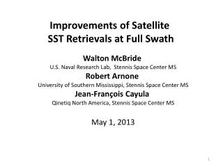
Improvements of Satellite SST Retrievals at Full Swath Walton McBride U.S. Naval Research Lab, Stennis Space Center MS Robert Arnone University of Southern Mississippi, Stennis Space Center MS Jean-François Cayula Qinetiq North America, Stennis Space Center MS May 1, 2013

A FRESH PERSPECTIVE Search for Clues on how to Improve SST Retrievals SST algorithms Used to Create Clues Scatter Plots Used to Identify Clues Model Run Results to Discern Clues Putting the Clues Together Interpretation of Results Conclusions

SST ALGORITHMS MC SST NL SST First guess temperature field Tfield SST (same as MC SST, except for addition of Tfield as separate predictor)

BUOY DATA SET NAVOCEANO buoy data set for the month of June 2012: 115,036 daytime points After routine NAVOCEANO filtering: 61,782 points from 0° to 53° zenith angle (53.70%) 97,496 points from 0° to 70° zenith angle (84.75%) Linear regression coefficients using MC SST: In the original spirit behind the MC SST formulation: where

SSTMC-T11 vs. T11-T12 Filtering Parameters |Tfield-Buoy| < 2.0° |Zenith| < 53 deg Ddistance < 25 km Dtime < 4 hours MCSST No scatter Pinch effect

BUOY-T11 vs. T11-T12 SSTMC-T11 vs. T11-T12 BUOY a Filtering Parameters |Tfield-Buoy| < 2.0° |Zenith| < 53 deg Ddistance < 25 km Dtime < 4 hours Data displays scatter Goal is to capture the features and structure of the distribution. No Pinch effect MCSST b No scatter Pinch effect

BUOY-T11 vs. T11-T12 SSTNL-T11 vs. T11-T12 BUOY a Filtering Parameters |Tfield-Buoy| < 2.0° |Zenith| < 53 deg Ddistance < 25 km Dtime < 4 hours Data displays scatter Goal is to capture the features and structure of the distribution. No Pinch effect MCSST NLSST c b No scatter Signs of scatter Pinch effect Pinch effect

Tfield AS SEPARATE PREDICTOR Clim K100 K10 Filtering Clim rmserror c1 + c5 |Tfield-Buoy| < 0.1 0.021 0.057 0.026 5.921 0.978 0.999 0.07175 |Tfield-Buoy| < 0.2 0.074 0.194 0.088 20.33 0.927 1.001 0.12447 |Tfield-Buoy| < 0.5 0.245 0.643 0.261 66.82 0.759 1.004 0.25600 |Tfield-Buoy| < 1.0 0.471 1.218 0.535 128.5 0.541 1.012 0.36675 |Tfield-Buoy| < 2.0 0.649 1.663 0.736 177.0 0.364 1.013 0.45077 |Tfield-Buoy| < 5.0 0.752 1.914 0.853 204.9 0.259 1.011 0.49914 K100 rmserror c1 + c5 |Tfield-Buoy| < 0.1 0.009 0.018 0.005 2.458 0.991 1.000 0.06968 |Tfield-Buoy| < 0.2 0.043 0.096 0.055 11.86 0.957 1.000 0.12447 |Tfield-Buoy| < 0.5 0.195 0.475 0.229 53.23 0.806 1.001 0.25554 |Tfield-Buoy| < 1.0 0.389 0.958 0.467 106.1 0.615 1.004 0.36104 |Tfield-Buoy| < 2.0 0.527 1.310 0.633 143.6 0.479 1.006 0.42815 |Tfield-Buoy| < 5.0 0.585 1.462 0.697 159.5 0.420 1.005 0.46373 K10 rmserror c1 + c5 |Tfield-Buoy| < 0.1 0.013 0.032 0.011 3.600 0.986 0.999 0.06991 |Tfield-Buoy| < 0.2 0.055 0.130 0.063 15.10 0.945 1.000 0.12362 |Tfield-Buoy| < 0.5 0.188 0.454 0.239 51.21 0.814 1.002 0.24467 |Tfield-Buoy| < 1.0 0.326 0.810 0.406 89.01 0.677 1.003 0.33348 |Tfield-Buoy| < 2.0 0.419 1.049 0.518 114.3 0.585 1.004 0.39268 |Tfield-Buoy| < 5.0 0.467 1.169 0.571 127.2 0.539 1.006 0.43082 Table1: Effects of pre-filtering and increased spatial resolution of Tfield.

Red Blue COLOR PLOTTING Blue Red COLOR PLOTTING b a DATA c d MC SST

Red Blue COLOR PLOTTING Blue Red COLOR PLOTTING b a DATA c d Tfield SST with K10

DEPENDENCE ON ZENITH ANGLE From GUI results |Zenith| Band #ptsrmserror bias c1 c2 c3 c4 c5 (c1+c5) +60 to +70 21213 0.41834 -8.37e-13 0.230 0.292 0.296 62.7 0.794 1.024 +50 to +60 19667 0.39780 -2.03e-13 0.296 0.621 0.349 80.9 0.721 1.017 +40 to +50 15353 0.39463 2.83e-13 0.343 0.814 0.447 93.4 0.665 1.008 +30 to +40 12415 0.38942 -9.51e-13 0.407 1.004 0.742 110.8 0.594 1.001 +20 to +30 10231 0.38372 -2.92e-12 0.469 1.264 -0.011 127.7 0.533 1.002 +10 to +20 9477 0.37942 7.47e-13 0.521 1.325 1.087 141.9 0.482 1.003 0 to +10 9151 0.37119 -6.32e-13 0.493 1.292 0.922 134.3 0.506 0.999 Using global coefficients 97507 0.41055 3.66e-12 0.294 0.610 0.388 80.10 0.719 1.013 no K10 0.65727 1.09e-11 1.034 2.204 1.363 281.8 0.000 1.034 |Zenith| Band #ptsrmserror bias rmserror bias +60 to +70 21213 0.44234 -0.04142 0.86911 -0.16031 +50 to +60 19667 0.39847 -0.00778 0.63142 0.01057 +40 to +50 15353 0.39828 0.00676 0.58992 0.05601 +30 to +40 12415 0.40274 0.02223 0.58093 0.06392 +20 to +30 10231 0.40334 0.01332 0.53541 0.05429 +10 to +20 9477 0.40560 0.03403 0.50201 0.06380 0 to +10 9151 0.39493 0.02127 0.52607 0.04228 Table 2: Coefficients Dependence on Zenith

DEPENDENCE ON LATITUDE From GUI results Latitude Band #ptsrmserror bias c1 c2 c3 c4 c5 (c1+c5) +50 to +70 7112 0.36861 -1.38e-12 0.375 0.980 0.314 102.2 0.626 1.001 +30 to +50 17404 0.39976 5.79e-13 0.513 1.191 0.626 139.8 0.497 1.010 +10 to +30 12910 0.3532 -6.44e-13 0.279 0.672 0.339 76.3 0.731 1.010 -10 to +10 4856 0.3521 -1.66e-13 0.242 0.795 0.240 63.9 0.672 0.914 -30 to -10 8947 0.34733 -1.81e-13 0.432 1.080 0.554 117.9 0.580 1.012 -50 to -30 9098 0.38322 -6.67e-13 0.514 1.054 0.612 140.0 0.501 1.015 -70 to -50 1468 0.36599 -2.07e-14 0.359 0.777 0.359 98.1 0.673 1.032 Using global coefficients 61795 0.3894 3.05e-12 0.416 1.039 0.515 113.4 0.589 1.005 no K10 0.5305 6.62e-12 1.006 2.550 1.174 274.1 0.000 1.006 Latitude Band #ptsrmserror bias rmserror bias +50 to +70 7112 0.37013 -0.02832 0.5056 -0.07924 +30 to +50 17404 0.40451 0.12566 0.51462 0.11358 +10 to +30 12910 0.36430 -0.01473 0.57448 -0.11061 -10 to +10 4856 0.38496 -0.11888 0.58587 -0.11294 -30 to -10 8947 0.34863 -0.07716 0.47300 0.00595 -50 to -30 9098 0.38908 -0.06359 0.49011 0.05780 -70 to -50 1468 0.37408 0.03549 0.47590 -0.00664 Table 3: Coefficients Dependence on Latitude, Zenith 0 to 53

RMS ERROR REDUCTION Zenith MCSST Tfield = ClimTfield = K100 Tfield = K10 0o to 53o 53o to 70o 0o to 70o 0.53052 0.45077 15.0%0.42551 19.8% 0.38937 26.6% 0.73712 0.51667 29.9% 0.45622 38.1% 0.41298 43.9% 0.65627 0.49989 23.8% 0.45507 30.7% 0.41053 37.4% Table 4: Percent reduction in rms error

ANOTHER CLUE! c1 c2 c3 c4 c5 rmserror 1.006 2.541 1.173 274.10 ---- 0.5058 0.251 0.617 0.312 68.42 0.752 0.2869 1.000 2.467 1.243 272.58 ---- MCSST TfieldSST Zenith angles from 0 to 53 degrees |Tfield-Tbuoy|=0.7° Clue 2: c1 c2 c3 c4 c5 rmserror 1.034 2.20 1.360 281.99 ---- 0.6382 0.163 0.326 0.221 44.48 0.844 0.2987 1.000 2.00 1.356 272.88 ---- MCSST TfieldSST Zenith angles from 0 to 70 degrees |Tfield-Tbuoy|=0.7°

PUTTING IT ALTOGETHER Clue 1: Clue 2: Substituting: Simple Linear Weighting or Present - Past Past If the errors in Tfield and SSTMC are uncorrelated, then the variances: where and

SCATTER PLOT OF ERRORS R2 < 0.04 PRACTICALLY NO CORRELATION! Zenith angles from 0 to 70 degrees Blue Red Color Plotting Red Blue Color Plotting

RMS ERRORS RELATIONSHIPS If the errors in Tfield and SSTMC are uncorrelated, then the variances are related as: Resistors in Parallel Analogy Guarantees that will always be less than or !

RMS ERRORS RELATIONSHIPS Interestingly, we have control of Tfieldrms error through more aggressive filtering. But at what price?

TRADE-OFF: rms error vs. # buoy data points SSTMC weakly affected by aggressive filtering Low Dropoff Stability Plot of rms error and % filtered points vs.|Tfield – Tbuoy| Zenith from 0 to 53

TRADE-OFF: rms error vs. # buoy data points SSTMC weakly affected by aggressive filtering Stability Low Dropoff Plot of rms error and % filtered points vs.|Tfield – Tbuoy| Zenith from 53 to 70

TRADE-OFF: rms error vs. # buoy data points SSTMC weakly affected by aggressive filtering Low Dropoff Stability Plot of rms error and % filtered points vs.|Tfield – Tbuoy| Zenith from 0 to 70

EVIDENCE OF REAL RMS ERROR REDUCTION Red Blue Color Plotting Blue Red Color Plotting MCSST TfieldSST with K10 Zenith from 0 to 53 |Tfield-Tbuoy| = 0.7

HELP ME UNDERSTAND, LENA! SSTMC

HELP ME UNDERSTAND, LENA! Tfield SSTMC + uncorrelated noise

HELP ME UNDERSTAND, LENA! Tfield SSTTfield SSTMC = + Always clearer image!

A FRESH PERSPECTIVE TWO-PRONGED IMPROVEMENT EFFORTS HARDWARE (2 or more looks) CLOUD MASK HIGH ZENITH ANGLES (emissivity, sea roughness) NAVOCEANO K100, K10, K2 IN SITU BUOY DATA Using Satellite Data Only!

CONCLUSIONS Although Tfield is used in NLSST, its additional information is tamed due to its appearance as a multiplier of T11-T12. Use of Tfield as a separate predictor results in a significant increase in accuracy for all existing SST algorithms, daytime and nighttime, due to resulting variance always being less. Tfield now is on equal footing with existing SST algorithms predicitions and improvements in its accuracy will benefit all combinations of existing SST algorithms and Tfield. TfieldSST algorithm was found to be extremely stable. Reduced to a formulation that leads to specific relationships between variances of MCSST and Tfield. NAVOCEANO’s Tfield characterizations, K100 and K10, only use previous satellitedata. NAVOCEANO is currently working on K2, at 2km resolution. TfieldSST algorithm allows for rms error under 0.3K over the full swath (0 to 70), while sacrificing a very modest number of buoy data points (from original 84.75%): 75% of buoy data points left from 0 to 70 with TfieldSST versus 55% of buoy data points left from from 0 to 53PRESENTLY

QUESTIONS ?

INCREASING Tfield IMPORTANCE a b Pinch effect moves to +1 Pinch effect Tdiffoffset = -1rmserror = 0.62069 Tdiffoffset = 0rmserror = 0.52546 c d Data • Pinch effect disappears • Scatter is more pronounced • rmserror diminishes Tdiffoffset = +10 rmserror = 0.44501 Tdiffoffset = +5rmserror = 0.45413 Adding Tdiffoffset to NLSST

Walton McBride U.S. Naval Research Lab, Stennis Space Center MS Robert Arnone