Download
1 / 52
560 likes | 1.07k Vues
Differential Equations. Objective: To solve a separable differential equation. Differential Equations. We will now consider another way of looking at integration. Suppose that f(x) is a known function and we are interested in finding a function F(x) such that y = F(x) satisfies the equation.

E N D
Differential Equations Objective: To solve a separable differential equation.
Differential Equations • We will now consider another way of looking at integration. Suppose that f(x) is a known function and we are interested in finding a function F(x) such that y = F(x) satisfies the equation
Differential Equations • We will now consider another way of looking at integration. Suppose that f(x) is a known function and we are interested in finding a function F(x) such that y = F(x) satisfies the equation • The solutions of this equation are the antiderivatives of f(x), and we know that these can be obtained by integrating f(x). For example, the solutions of the equation are
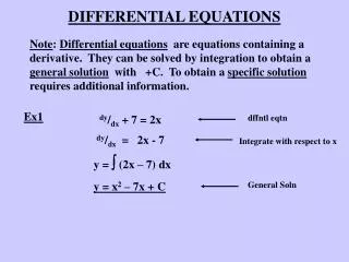
Differential Equations • An equation of the form is called a differential equation because it involves a derivative of an unknown function. Differential equations are different from kinds of equations we have encountered so far in that the unknown is a function and not a number.
Differential Equations • Sometimes we will not be interested in finding all of the solutions of the equation, but rather we will want only the solution whose integral curve passes through a specified point.
Differential Equations • Sometimes we will not be interested in finding all of the solutions of the equation, but rather we will want only the solution whose integral curve passes through a specified point. • For simplicity, it is common in the study of differential equations to denote a solution of as y(x) rather than F(x), as earlier. With this notation, the problem of finding a function y(x) whose derivative is f(x) and whose integral curve passes through the point (x0, y0) is expressed as
Differential Equations • Equations of the form are known as initial value problems, and is called the initial condition for the problem.
Differential Equations • Equations of the form are known as initial value problems, and is called the initial condition for the problem. • To solve an equation of this type, first we will separate the variables, integrate, and solve for C.
Example • Solve the initial-value problem
Example • Solve the initial-value problem • Separate the variables
Example • Solve the initial-value problem • Separate the variables • Integrate
Example • Solve the initial-value problem • Separate the variables • Integrate • Solve for C
Example 1 • Solve the initial-value problem
Example 1 • Solve the initial-value problem • Separate the variables
Example 1 • Solve the initial-value problem • Separate the variables • Integrate
Example 1 • Solve the initial-value problem • Separate the variables • Integrate • Solve for C
Example 1 • Solve the initial-value problem • Separate the variables • Integrate • Solve for C
Example 2 • Solve the initial-value problem
Example 2 • Solve the initial-value problem • Separate the variables
Example 2 • Solve the initial-value problem • Separate the variables • Integrate
Example 2 • Solve the initial-value problem • Separate the variables • Integrate • Solve for C
Example 3 • Find a curve in the xy-plane that passes through (0,3) and whose tangent line at a point has slope .
Example 3 • Find a curve in the xy-plane that passes through (0,3) and whose tangent line at a point has slope . • Since the slope of the tangent line is dy/dx, we have
Example 3 • Find a curve in the xy-plane that passes through (0,3) and whose tangent line at a point has slope . • Since the slope of the tangent line is dy/dx, we have
Example 3 • Find a curve in the xy-plane that passes through (0,3) and whose tangent line at a point has slope . • Since the slope of the tangent line is dy/dx, we have
Example • Solve the differential equation
Example • Solve the differential equation • Separate the variables
Example • Solve the differential equation • Separate the variables • Integrate
Example • Solve the differential equation • Separate the variables • Integrate • Solve for y
Example • Solve the differential equation • Separate the variables • Integrate • Solve for y
Exponential Growth and Decay • Population growth is an example of a general class of models called exponential models. In general, exponential models arise in situations where a quantity increases or decreases at a rate that is proportional to the amount of the quantity present. This leads to the following definition:
Exponential Growth and Decay • Equations 10 and 11 are separable since they have the right form, but with t rather than x as the independent variable. To illustrate how these equations can be solved, suppose that a positive quantity y = y(t) has an exponential growth model and that we know the amount of the quantity at some point in time, say y = y0 when t = 0. Thus, a formula for y(t) can be obtained by solving the initial-value problem
Exponential Growth and Decay • Equations 10 and 11 are separable since they have the right form, but with t rather than x as the independent variable. To illustrate how these equations can be solved, suppose that a positive quantity y = y(t) has an exponential growth model and that we know the amount of the quantity at some point in time, say y = y0 when t = 0. Thus, a formula for y(t) can be obtained by solving the initial-value problem
Exponential Growth and Decay • The initial condition implies that y = y0 when t =0. Solving for C, we get
Exponential Growth and Decay • The initial condition implies that y = y0 when t =0. Solving for C, we get
Exponential Growth and Decay • The significance of the constant k in the formulas can be understood by reexamining the differential equations that gave rise to these formulas. For example, in the case of the exponential growth model, we can rewrite the equation as which states that the growth rate as a fraction of the entire population remains constant over time, and this constant is k. For this reason, k is called the relative growth rate.
Example 4 • According to United Nations data, the world population in 1998 was approximately 5.9 billion and growing at a rate of about 1.33% per year. Assuming an exponential growth model, estimate the world population at the beginning of the year 2023.
Example 4 • According to United Nations data, the world population in 1998 was approximately 5.9 billion and growing at a rate of about 1.33% per year. Assuming an exponential growth model, estimate the world population at the beginning of the year 2023.
Doubling Time and Half-Life • If a quantity has an exponential growth model, then the time required for the original size to double is called the doubling time, and the time required to reduce by half is called the half-life. As it turns out, doubling time and half-life depend only on the growth or decay rate and not on the amount present initially.
Example 5 • It follows that form the equation that with a continued growth rate of 1.33% per year, the doubling time for the world population will be
Radioactive Decay • It is a fact of physics that radioactive elements disintegrate spontaneously in a process called radioactive decay. Experimentation has shown that the rate of disintegration is proportional to the amount of the element present, which implies that the amount y = y(t) of a radioactive element present as a function of time has an exponential decay model.
Radioactive Decay • It is a fact of physics that radioactive elements disintegrate spontaneously in a process called radioactive decay. Experimentation has shown that the rate of disintegration is proportional to the amount of the element present, which implies that the amount y = y(t) of a radioactive element present as a function of time has an exponential decay model. The half life of carbon-14 is 5730 years. The rate of decay is:
Example 6 • If 100 grams of radioactive carbon-14 are stored in a cave for 1000 years, how many grams will be left at that time?
Example 6 • If 100 grams of radioactive carbon-14 are stored in a cave for 1000 years, how many grams will be left at that time?
Carbon Dating • When the nitrogen in the Earth’s upper atmosphere is bombarded by cosmic radiation, the radioactive element carbon-14 is produced. This carbon-14 combines with oxygen to form carbon dioxide, which is ingested by plants, which in turn are eaten by animals. In this way all living plants and animals absorb quantities of radioactive carbon-14. In 1947 the American nuclear scientist W. F. Libby proposed that
Carbon Dating • In 1947 the American nuclear scientist W. F. Libby proposed the theory that the percentage of carbon-14 in the atmosphere and in living tissues of plants is the same. When a plant of animal dies, the carbon-14 in the tissue begins to decay. Thus, the age of an artifact that contains plant or animal material can be estimated by determining what percentage of its original carbon-14 remains. This is called carbon-dating or carbon-14 dating.
Example 7 • In 1988 the Vatican authorized the British Museum to date a cloth relic know as the Shroud of Turin, possibly the burial shroud of Jesus of Nazareth. This cloth, which first surfaced in 1356, contains the negative image of a human body that was widely believed to be that of Jesus.
Example 7 • The report of the British Museum showed that the fibers in the cloth contained approximately 92% of the original carbon-14. Use this information to estimate the age of the shroud.