Download
1 / 85
900 likes | 1.3k Vues
Doctoral Defence. Characterization, Modelling and Control of Mechanical Systems Comprising Material and Geometrical Nonlinearities. Tegoeh Tjahjowidodo Katholieke Universiteit Leuven Departement Werktuigkunde, Div. PMA Thursday 16 November 2006. Overview. Introduction

E N D
Doctoral Defence Characterization, Modelling and Control of Mechanical Systems Comprising Material and Geometrical Nonlinearities Tegoeh Tjahjowidodo Katholieke Universiteit Leuven Departement Werktuigkunde, Div. PMA Thursday 16 November 2006
Overview • Introduction • Nonlinearity sources • Dynamic signal classification • Geometric Nonlinearity (Backlash) • Material Nonlinearity (Friction) • Control of Nonlinear Systems • Application on a Real System Mechanical Systems with Harmonic Drive elements • Conclusions • Introduction • Nonlinearity sources • Dynamic signal classification • Geometric Nonlinearity (Backlash) • Material Nonlinearity (Friction) • Control of Nonlinear Systems • Application on a Real System Mechanical Systems with Harmonic Drive elements • Conclusions • Introduction • Nonlinearity sources • Dynamic signal classification • Geometric Nonlinearity (Backlash) • Material Nonlinearity (Friction) • Control of Nonlinear Systems • Application on a Real System Mechanical Systems with Harmonic Drive elements • Conclusions • Introduction • Nonlinearity sources • Dynamic signal classification • Geometric Nonlinearity (Backlash) • Material Nonlinearity (Friction) • Control of Nonlinear Systems • Application on a Real System Mechanical Systems with Harmonic Drive elements • Conclusions • Introduction • Nonlinearity sources • Dynamic signal classification • Geometric Nonlinearity (Backlash) • Material Nonlinearity (Friction) • Control of Nonlinear Systems • Application on a Real System Mechanical Systems with Harmonic Drive elements • Conclusions • Introduction • Nonlinearity sources • Dynamic signal classification • Geometric Nonlinearity (Backlash) • Material Nonlinearity (Friction) • Control of Nonlinear Systems • Application on a Real System Mechanical Systems with Harmonic Drive elements • Conclusions Geometric Nonlinearity Material Nonlinearity Control of Nonlinear Systems Application on Real System Conclusions Introduction • Introduction • Nonlinearity sources • Dynamic signal classification • Geometric Nonlinearity (Backlash) • Material Nonlinearity (Friction) • Control of Nonlinear Systems • Application on a Real System Mechanical Systems with Harmonic Drive elements • Conclusions
Introduction • Motivation: Having better understanding of a system via appropriate techniques System Identification ! Introduction Geometric Nonlinearity Material Nonlinearity Control of Nonlinear Systems Application on Real System Conclusions • Identification purposes: • Dynamic behaviour analysis • Design engineering • Damage detection • Control design • There is no general identification method applicable to all systems. this depends on the characteristic of the system and the type of the signal involved in the identification. • Control design
Characteristic of systems Force B.C prescribed displacement (û) body force (b) displacement (u) Displacement B.C. Geometric nonlinearity prescribed forces (t) strain (e) stress (σ) Material nonlinearity Nonlinearity in a mechanical system can be attributed to different sources: Introduction Geometric Nonlinearity Material Nonlinearity Control of Nonlinear Systems Application on Real System Conclusions
Geometrical and Material Nonlinearities • Geometric Nonlinearity • the change in geometry as the structure deforms causes a nonlinear change of the parameters in the system • hardening spring, softening spring, saturation, … • Material Nonlinearity • the behaviour of material depends on the current deformation • frictional losses, ferromagnetism Introduction Geometric Nonlinearity Material Nonlinearity Control of Nonlinear Systems Application on Real System Conclusions
Dynamic Signal Classification Dynamic Signal Deterministic ‘Well-behaved’ • Chaotic: • Lyapunov Exponent • Correlation Dimension • etc Random Stationary: • Frequency Response Function • Volterra • etc Non-stationary: • Short Time Fourier Transform • Wigner-Ville • Wavelet • Hilbert In general dynamic signals can be classified: Introduction Geometric Nonlinearity Material Nonlinearity Control of Nonlinear Systems Application on Real System Conclusions
Geometric Nonlinearity x0 Fin x k1x+F(x) k0 m k1+ k0 c k1 k1 -x0 x0 x Case study: mechanical system with backlash element Introduction Geometric Nonlinearity •Well-behaved •Chaotic Material Nonlinearity Control of Nonlinear Systems Application on Real System Conclusions Backlash: In a mechanical system, any lost motion between driving and driven elements due to clearance between parts.
Backlash Two different cases might appear: Introduction Geometric Nonlinearity •Well-behaved •Chaotic Material Nonlinearity Control of Nonlinear Systems Application on Real System Conclusions • ‘well-behaved’ response for periodic input • Skeleton identification • Hilbert transform • Wavelet analysis • chaotic response for periodic input • Chaos quantification • Lyapunov exponent • Surrogate Data Test
Skeleton identification SDOF system: y(t) = A(t)·cos [y(t)-f] • Free vibration response can be represented in the combination of envelope and instantaneous phase. Introduction Geometric Nonlinearity • Well-behaved •Chaotic Material Nonlinearity Control of Nonlinear Systems Application on Real System Conclusions
Skeleton identification Introduction Geometric Nonlinearity • Well-behaved •Chaotic Material Nonlinearity Control of Nonlinear Systems Application on Real System Conclusions Envelope and instantaneous phase of the free vibration response can be used as a mechanical signature of the dynamic parameters of the system (Feldman 1994a).
Skeleton signature examples (1) Signatures of restoring forces Introduction Geometric Nonlinearity • Well-behaved •Chaotic Material Nonlinearity Control of Nonlinear Systems Application on Real System Conclusions
Skeleton signature examples (2) Signatures of damping forces Introduction Geometric Nonlinearity • Well-behaved •Chaotic Material Nonlinearity Control of Nonlinear Systems Application on Real System Conclusions
Parameters identification Feldman (1994a) formulated parameters of the system based on the instantaneous envelope and phase: Introduction Geometric Nonlinearity • Well-behaved •Chaotic Material Nonlinearity Control of Nonlinear Systems Application on Real System Conclusions Extending the method to forced vibration problem, Feldman (1994b) proposed the following relations:
Instantaneous information extraction (1) ~ y(t) = A(t)·sin [y(t)-f] HT Analytic Signal of y(t) [z(t)] |z(t)| • Hilbert transform: a mathematical transform that shift each frequency component of the instantaneous spectrum by p/2 without affecting the magnitude. Introduction Geometric Nonlinearity • Well-behaved •Chaotic Material Nonlinearity Control of Nonlinear Systems Application on Real System Conclusions y(t) = A(t)·cos [y(t)-f] (+) simple, fast, practical (–) inaccurate! (only suitable for asympotic signal)
Wavelet transform: Instantaneous information extraction (2) instantaneous frequency (in dilation form): envelope in modulus of wavelet: a time-frequency representation (TFR) technique Introduction Geometric Nonlinearity • Well-behaved •Chaotic Material Nonlinearity Control of Nonlinear Systems Application on Real System Conclusions (Complex Morlet Wavelet) (+) accurate! (–) time consuming, error at the edges, cumbersome
Illustration of extraction Envelope Estimation Instantaneous Frequency Estimation 1.5 20 HT technique HT technique Wavelet technique Wavelet technique 15 1 10 0.5 Amplitude Frequency 5 0 0 -0.5 -5 -1 -10 0 2 4 6 8 10 0 2 4 6 8 10 time (s) time (s) Damped-chirp signal Introduction Geometric Nonlinearity • Well-behaved •Chaotic Material Nonlinearity Control of Nonlinear Systems Application on Real System Conclusions
Experimental Setup 2nd link Encoder #2 Encoder #1 1st link Schematic drawing of a two-link mechanism Introduction Geometric Nonlinearity • Well-behaved •Chaotic Material Nonlinearity Control of Nonlinear Systems Application on Real System Conclusions • 1st link fixed • backlash was introduced in the joint • considered as a base motion system
Base Motion System k m c y x Introduction Geometric Nonlinearity • Well-behaved •Chaotic Material Nonlinearity Control of Nonlinear Systems Application on Real System Conclusions where z is a relative motion between x and y Force balance diagram of link #2 q : displacement input f : displacement output
Displacement Input Displacement input measured by encoder #1 Introduction Geometric Nonlinearity • Well-behaved •Chaotic Material Nonlinearity Control of Nonlinear Systems Application on Real System Conclusions Input (degree) time (s)
Displacement Output Output (degree) time (s) Displacement output measured by encoder #2 Introduction Geometric Nonlinearity • Well-behaved •Chaotic Material Nonlinearity Control of Nonlinear Systems Application on Real System Conclusions
Relative Motion Relative motion (degree) Backlash size time (s) Relative motion between output and input(f-q) Introduction Geometric Nonlinearity • Well-behaved •Chaotic Material Nonlinearity Control of Nonlinear Systems Application on Real System Conclusions
Envelope and Instantaneous Frequency (1) Envelope and instantaneous frequency estimation of input signal using Hilbert and Wavelet Transform Introduction Geometric Nonlinearity • Well-behaved •Chaotic Material Nonlinearity Control of Nonlinear Systems Application on Real System Conclusions Instantaneous frequency extraction Envelope extraction Frequency (Hz) time (s) time (s)
Envelope and Instantaneous Frequency (2) Envelope and instantaneous frequency estimation of output signal using Hilbert and Wavelet Transform Introduction Geometric Nonlinearity • Well-behaved •Chaotic Material Nonlinearity Control of Nonlinear Systems Application on Real System Conclusions Instantaneous frequency extraction Envelope extraction Frequency (Hz) time (s) time (s)
Restoring force estimation Reconstruction of restoring force using Hilbert and Wavelet Transform Introduction Geometric Nonlinearity • Well-behaved •Chaotic Material Nonlinearity Control of Nonlinear Systems Application on Real System Conclusions
Damping force estimation Reconstruction of damping force using Hilbert and Wavelet Transform Introduction Geometric Nonlinearity • Well-behaved •Chaotic Material Nonlinearity Control of Nonlinear Systems Application on Real System Conclusions
Identification on Well-behaved Case Introduction Geometric Nonlinearity • Well-behaved •Chaotic Material Nonlinearity Control of Nonlinear Systems Application on Real System Conclusions Wavelet transform offers better results than the Hilbert transform in skeleton method.
Chaoticity in a system with backlash Schematic of mechanical system with backlash component Introduction Geometric Nonlinearity • Well-behaved • Chaotic Material Nonlinearity Control of Nonlinear Systems Application on Real System Conclusions Example of parameters that lead to chaotic motion:
Chaotic response (1) CASE 1 was excited with sinusoidal signal with A=100 N and w=40 rad/s Introduction Geometric Nonlinearity • Well-behaved • Chaotic Material Nonlinearity Control of Nonlinear Systems Application on Real System Conclusions Displacement (mm) Power spectrum (dB) Freq. (Hz) time (s)
Chaotic response (2) Phase plot Poincaré map velocity (mm/s) velocity (mm/s) displacement (mm) displacement (mm) Phase plot and Poincaré map of case 1 Introduction Geometric Nonlinearity • Well-behaved • Chaotic Material Nonlinearity Control of Nonlinear Systems Application on Real System Conclusions
Chaos Identification EXPONENTIAL GROWTH dt • for exponential growth, should see • is the average rate of the exponential growth • Lyapunov exponent d = d e lt 0 t How do we know when the mapping is chaotic? quantification of chaos Lyapunov exponents Introduction Geometric Nonlinearity • Well-behaved • Chaotic Material Nonlinearity Control of Nonlinear Systems Application on Real System Conclusions • consider one dimension: • take two initial conditions differing by a small amount • to identify chaos, observe the evolution in time and compare the differences ▪▪ TWO NEARBY INITIAL TRAJECTORY d0
Dimensional Analysis In order to examine the influence of each parameter on the nature of resulting response Introduction Geometric Nonlinearity • Well-behaved • Chaotic Material Nonlinearity Control of Nonlinear Systems Application on Real System Conclusions where: primes indicate differentiation with respect to .
Effect of Forcing Parameter and Backlash Largest Lyapunov Exponent 1/a=3.4 1/a 1/a=4.6 Lyapunov exponent vs Forcing Parameter and/or Backlash Size Introduction Geometric Nonlinearity • Well-behaved • Chaotic Material Nonlinearity Control of Nonlinear Systems Application on Real System Conclusions
Chaotic response in experimental setup Phase plots of output responses for periodic signal with different excitation level Introduction Geometric Nonlinearity • Well-behaved • Chaotic Material Nonlinearity Control of Nonlinear Systems Application on Real System Conclusions
Noise Reduction in Chaotic Signal • Simple Noise Reduction Method • developed based on near future prediction Introduction Geometric Nonlinearity • Well-behaved • Chaotic Material Nonlinearity Control of Nonlinear Systems Application on Real System Conclusions Phase plots of output responses for periodic signal before and after noise reduction
Noise Effect in Estimating Dimension Minimum embedding dimension information for phase-plot reconstruction Introduction Geometric Nonlinearity • Well-behaved • Chaotic Material Nonlinearity Control of Nonlinear Systems Application on Real System Conclusions
Identification on Chaotic Case Introduction Geometric Nonlinearity • Well-behaved • Chaotic Material Nonlinearity Control of Nonlinear Systems Application on Real System Conclusions Observing the chaos quantifier, e.g. Lyapunov exponent, could be used, in principle, to estimate the parameter of a system.
Material Nonlinearity friction velocity Case study: mechanical system with friction element Introduction Geometric Nonlinearity Material Nonlinearity Control of Nonlinear Systems Application on Real System Conclusions Friction is the result of a complex interaction between two contact surfaces. • Conventional friction model: Coulomb model • discontinuity at zero velocity
Friction Characterisation Two different friction regimes have been distinguished: Introduction Geometric Nonlinearity Material Nonlinearity Control of Nonlinear Systems Application on Real System Conclusions • the pre-sliding regime: appears predominantly as a function of displacement • the sliding regime: function of sliding velocity (Armstrong-Hélouvry, 1991, Canudas de Wit et al., 1995, Swevers et al., 2000, Al-Bender et al., 2004)
Pre-sliding regime (1) Friction force Fm 1 1 3 y(q) 2 -qm qm 0 (displacement) x -y(-q) y(q) 2 2 x Pre-sliding friction • Friction force in pre-sliding regime not only depends on the output at some time instant in the past and the input, but also on past extremum values of the input or output as well. hysteresis with non-local memory Introduction Geometric Nonlinearity Material Nonlinearity Control of Nonlinear Systems Application on Real System Conclusions 4
Pre-sliding regime (2) friction displacement Equivalent dynamic parameters The Describing Function technique is used to obtain the equivalent stiffness and damping: Introduction Geometric Nonlinearity Material Nonlinearity Control of Nonlinear Systems Application on Real System Conclusions y(q) is the virgin curve of the hysteresis
Pre-sliding friction model F Wi ki x • Alternative representation of hysteresis function with non-local memory for pre-sliding friction: parallel connection of N elasto-slide elements (Maxwell-Slip elements) Introduction Geometric Nonlinearity Material Nonlinearity Control of Nonlinear Systems Application on Real System Conclusions
Sliding regime • When the motion is entering the sliding regime, in most cases, the Maxwell-Slip model is no longer suitable. Introduction Geometric Nonlinearity Material Nonlinearity Control of Nonlinear Systems Application on Real System Conclusions • The friction usually has a maximum value at the beginning and then continues to decrease with increasing velocity
GMS friction model • Generalized Maxwell-Slip (GMS) model • developed at PMA/KULeuven Introduction Geometric Nonlinearity Material Nonlinearity Control of Nonlinear Systems Application on Real System Conclusions • If the model is sticking: Mathematical representation of Maxwell-Slip elements • If the model is slipping:
DC Motor dSPACE® 1104 acquisition board servo DC Motor amp Experimental setup of DC motor ABB M19-S Introduction Geometric Nonlinearity Material Nonlinearity Control of Nonlinear Systems Application on Real System Conclusions Encoder Load Timing Belt
Friction Identification • Two sets of experiments were carried out for friction identification in the DC motor (ABB M19-S): • Low frequencies signal • High frequencies signal Introduction Geometric Nonlinearity Material Nonlinearity Control of Nonlinear Systems Application on Real System Conclusions 1st velocity signal 2nd velocity signal velocity (rad/s) time (s) time (s)
Identification Strategy The optimization is based upon minimization of cost function: Introduction Geometric Nonlinearity Material Nonlinearity Control of Nonlinear Systems Application on Real System Conclusions Identification technique for the physics-based model: • Genetic Algorithm • Nelder-Mead Downhill Simplex Method
Identification Results #1 2.06% (0.3360) Coulomb model Exponential Coulomb model GMS 1.97% (0.3470) torque (Nm) MSE (max.err.) Coulomb 2.06% (0.3770) Exp-Coulomb LuGre 2.03% (0.3530) GMS model LuGre model torque (Nm) time (s) time (s) • Identification results of low frequencies experiment: Introduction Geometric Nonlinearity Material Nonlinearity Control of Nonlinear Systems Application on Real System Conclusions
Identification Results #2 Exponential Coulomb model Coulomb model 9.59% (1.2604) torque (Nm) GMS4 1.39% (0.5711) MSE (max.err.) Coulomb 17.92% (1.2993) Exp-Coulomb GMS model LuGre model LuGre 4.30% (0.6466) GMS10 1.19% (0.5177) torque (Nm) time (s) • Identification results of high frequencies experiment: Introduction Geometric Nonlinearity Material Nonlinearity Control of Nonlinear Systems Application on Real System Conclusions time (s)