Download
1 / 26
260 likes | 414 Vues
Towards a consolidated turbulence and surface coupling for COSMO and ICON:. Technical issues preparing the common module for COSMO and ICON Revision of security limits and the problem with the stable boundary layer (SBL) Foreseen modifications within the first PT ConSAT. Sibiu 2013. COSMO.

E N D
Towards a consolidated turbulence and surface coupling for COSMO and ICON: • Technical issues preparing the common module for COSMO and ICON • Revision of security limits and the problem with the stable boundary layer (SBL) • Foreseen modifications within the first PT ConSAT Sibiu 2013 COSMO Matthias Raschendorfer
Some technical issues preparing the common module: Requirement by ICON design • Call of organize_turbdiff by a long parameter list • Only one horizontal index of variable fields • Extraction of horizontal operations from the turbulence code • Horizontal shear; interpolations due to grid staggering • Stronger modularization (common subroutines for turbdiff and turbtran) • moist physics; turbulence model; initialization • Removing obsolete parts of the code • Different options for gaining positive definiteness of TKE, avoiding singularities in solution for stability functions and other security limits for future testing (stable boundary, SAT) • Trying to generate a somehow more systematic logic of switches and options More flexibility to adapt to hardware architecture Due to different horizontal ICON grid Clearer code structure; extensions easier to apply Facilitating future testing (SBL) More user friendly for testing procedure DWD Matthias Raschendorfer COSMO Sibiu 2013
Some technical issues preparing the common module: • Treating implicit vertical diffusion as a part of the turbulence module • Using a common subroutine for all species • Including half-level variables (TKE) • Including passive tracers • Allowing treatment of non-gradient fluxes in the same framework • Options for treatment of explicit tendencies • Optional preconditioning • Options for the treatment of the lower boundary (input of explicit surface fluxes possible) • In case of surface tiles: flux aggregation (tile structure outside the turbdiff module so far) • Diffusion of conserved variables and subsequent turbulent saturation adjustment possible Easier exchange of complete turbulence/diffusion framework Code is much easier to handle; avoiding code repetitions Facilitates testing the effect of different numerical treatment Forcing with prescribed surface fluxes possible Common tile structure not yet defined Easiest way to consider turbulent condensation in GS budgets • Mainly present in ICON; a private test version with 2 horizontal indices exists • Strategy: Generating interface for COSMO and using ICON-Module for further development!! DWD Matthias Raschendorfer COSMO Sibiu 2013
The problem with the stable boundary layer (SBL): • Almost no production term in a classical TKE equation almost no vertical mixing even though it is usually present in nature complete decoupling of the surface vertical shear by the mean flow buoyancy dissipation almost no dissolution of fog and inversion layer clouds almost zero for low wind conditions negative for downward heat flux always a sink singularities in turbulence model model solution is strongly dependent on numerical details considerable problems with numerical stability DWD Matthias Raschendorfer CUS 2013
Possible solutions of the problem: • Introduction of artificial background mixing • minimal value of TKE • restriction of thermal stability • minimal value for turbulent diffusion coefficients (tkm[m,h]min) momentum scalars (heat) • Problems with these measures • not physically based (except some additional laminar diffusion) • often too much mixing in the lower nocturnal BL • either too fast or too slowly dissolution of inversion layer clouds • either too strong or too weak nocturnal temperature decrease at the surface • danger of smoothing out vertical jet structure (e.g. of the low level jet) • Alternatives • Adopted numerical schemes • inherentvertical smoothingwithout explicit minimal diffusion coefficients • prognostic TKE equation guaranteeing positive definiteness without explicit limits Ready in test version and ICON DWD Matthias Raschendorfer CUS 2013
Physical based solution In official version; only wake production runs operational so far • Introduction of additional turbulence productionvia scale interaction • thermal density circulations; wake production; horizontal shear • Deardorff-reduction of the turbulent length scale • Turbulent transport of turbulent scalar variances (TKESV) • Considering circulation transport of GS and turbulent • Considering turbulent condensation in GS budgets In official version; verification has been delayed In test version; needs to be introduced as an option verified against current development not yet implemented GS saturation adjustment needs to be substituted by statistical approach including turbulence ad convection • More physical based TKE and mixing in the stable BL • Additional TKE sources are already beneficial for EDR-forecast (for aviation) • Should be beneficial for near surface SBL as well. • Previous artificial security measures needs to be adopted! • First candidate: the minimal diffusion coefficient • Previous value: tkv[h,m]min = 1.0 m2/s (same for scalars and momentum) • Seems to dissolve BL clouds much to early now (and was presumably always a bit too large) • Previous attempts to decrease it has not been successful. • After lots of general numerical improvement of the model and the introduction of the SSO-source term a further attempt has now been tried: New value: tkv[h,m]min = 0.4 m2/s DWD Matthias Raschendorfer CUS 2013
Low level cloud cover CLCL s Experiment Routine
diffusion-coefficient/[m2/s]: Routine Experiment time-height cut TKE/[m2/s2] TKE/[m2/s2] all values are area averages
cloud-water-content/[Kg/Kg]: Routine Experiment time-height cut Vel/[m/s] Theta/[°C] all values are area averages
Experiment - Routine Experiment - Routine time-height cut now more TKE (within the clouds) before more TKE: Initiating cloud dissolution before moister now moister all values are area averages
vertical profile now cooler day-time BL all values are area averages Experiment Routine now much more BL clouds now more intense low level jet
Conclusion: • In the SBL pure turbulence would completely disappear, unless non-turbulent sub-grid processes are interacting. • Introduction of scale interaction terms was the reason that previous security measures for the SBL could and must be degraded. • Reduction of tkv[h,m]min diminishes excessive dissolution of inversion layer clouds that seemed to get increasingly worse lately and causes more BL clouds now. • Less often completely wrong simulation of BL clouds • cooler BL also during daytime => slightly negative BIAS of T2m_max • we expect also less systematic radiative cooling of the soil during winter time (needs to be verified; experiment has been canceled due to technical problems) • Reduction of tkv[h,m]min diminishes night-time heat transfer towards the soil. • cooler clear sky surface layer during night => reduction of positive BIAS of T2m_min • Operational at DWD since December 2012 DWD Matthias Raschendorfer CUS 2013
Next steps: • Investigation of the other security measures in the scheme • Reformulation of the numerical sub schemes to allow for less restrictions (ready in a test version) • Less restrictive security measures to avoid singularities in the turbulent budget equations (ready in a test version) • Testing/Adapting/Verification of various implementations • The not yet activated scale interaction terms (by convection and horizontal shear) (ready in official version) • Deardorff-restriction of turbulent length scale for stable stratification (ready in official version) • Turbulent transport of scalar variances (TKESV) (ready in test version; to be adapted to official code as an option) • Turbulent saturation adjustment in grid scale budgets (in principle already possible) • Further development of the scheme • Reformulation of the thermal circulation term into a thermal SSO-source term (prepared) • Implementation of missing circulation transport of GS and turbulent properties (additional non-gradient diffusion) • Reformulation of the surface-to-atmosphere transfer in order to be more sensitive • for stable stratification (ConSAT) • Strategy: Generating interface for COSMO and using ICON-Module for further development!! DWD Matthias Raschendorfer CUS 2013
Specific problems of SAT: roughnesslayer earth • Close to the surface 2 additional difficulties arise: • Laminar diffusion can’t be neglected • Roughness layer effects (SGS terms due to non-linearity of spatial differentiation): • form drag • effect of increased surface • modification of turbulent length scale displacement height roughness length • Above the laminar layer, where molecular diffusion is negligible and above the roughness layer it holds: • The total effective vertical flux density can be written as: turbulent length scale squared surface area index molecular diffusion coefficient effective velocity scale pure turbulent velocity scale • It is only laminar diffusion at the surface DWD Matthias Raschendorfer CLM-Training Course
The constant flux layer: • Vertical gradientsincrease significantly approaching the surface. • Therefore the vertical profile of is not linear and can only be determined using further information. • In our model we assume that does not change significantly within the transfer layer between the surface and the lowest full model level . constant flux layer • Integration yields: transfer layer resistance squared surface area index roughness layer resistance free atmospheric resistance turbulent velocity scale specific roughness length DWD Matthias Raschendorfer CLM-Training Course
Transfer scheme and 2m-values with respect to a SYNOP lawn: SYNOP station lawn profile Effective velocity scale profile Mean GRID box profile upper boundary of the lowest model layer from turbulence-scheme linear interpolated logarithmic Prandtl-layer profile unstable stable lowest model main level (expon. roughness-layer profile) Prandtl layer lower boundary of the lowest model layer no storage capacity roughness layer laminar layer • Exponentialroughness layer profile is valid for the whole grid box, • but it is not present at a SYNOP station turbulence-scheme DWD Matthias Raschendorfer CLM-Training Course
Calculation of the transport resistances: • The current scheme in COSMOexplicitly considers the roughness layer resistance for scalars: for the whole roughness layer and an effective SAI value • applying and a proper scaling factor for scalars • using the laminar length scale for • assuming , it can be written: • Can be expressed by surface layer variables only, increasing sensitivity on thermal stratification • The current scheme in COSMOexplicitly considers the free atmospheric resistance: • applying a linear -profile between level (top of the roughness layer) (top of the lowest model layer) and level • using the atmospheric height and the stability parameter it can be written: new branch DWD May.2013 Matthias Raschendorfer
Next steps: • Investigation of numerical security limits in the related turbulence model • Implementation, verification and documentation of the revised transfer formulation • Detailed investigation of the problems with daily cycle of near surface variables using measurements and COSMO-SC 1-st 1-year task For longer terms: • Extension of the profile function towards an universal one that includes the laminar limit, thus getting rid of using a virtual laminar layer. • Revision of near surface diagnostics in particular with respect to their applicability at grid points with a large roughness length. • Implementation of the vertically resolved roughness layer with roughness terms in all 1-st and second order budgets and considering only the not resolved part in the SAT scheme (reduction of roughness length). DWD Matthias Raschendorfer COSMO Sibiu 2013
The general valid resistance: pure neutral contribution analytically integrable dimensionless resistance contribution with pure turbulent profile function contribution for additional laminar correction and from TKE scheme lowest full level Offenbach 2009 COSMO Matthias Raschendorfer
Normalized transition profile for wind speed: turbulent solution molecular solution according classical measurements form Reichardt 1951 according approximation Offenbach 2009 COSMO Matthias Raschendorfer
filtered topography For any scale Offenbach 2009 COSMO Matthias Raschendorfer
Roughness layer properties and the surface flux density: roughnesslayer earth -surfaces normal to localturbulent and molecular flux densities, being a shifted topographywithoutsmall scale modesnot contributing to for any variable . Their area is times the horizontal projection • Above the roughness layer, the surface area index is equal to 1 and can be chosen so that it holds there: mean distance form the rigid surface von Kaman constant • At the lowest level, where this is valid, it is: displacement height roughness length • Using can be described in the roughness layer and • The flux densities of prognostic model variables at the lower model boundary are affected by the roughness layer and have turbulent as well as molecular contributions: • Above the laminar layer, where molecular diffusion is negligible and above the roughness layer it holds: • The total effective vertical flux density can be written as: turbulent length scale squared surface area index molecular diffusion coefficient effective velocity scale pure turbulent velocity scale • It is only laminar diffusion at the surface DWD Matthias Raschendorfer CLM-Training Course
Further development: • Switching on the implemented scale interaction terms after verification against SYNOP data (operational verification) • Reformulation of the surface induced density flow term (circulation term) in the current scheme to become a thermal SSO production dependent on SSO parameters • Expression of direct sub grid scale transport by SSO eddies and horizontal shear eddies • Introduction of an option for three additional prognostic scalar variance equations (UCTS) • Detailed investigation of the problems with daily cycle of near surface variables using measurements and COSMO-SC (ConSAT) • Implementation and verification of the full revised transfer formulation (ConSAT) • Implicit calculation of surface temperature by liniarized surface energy budget, including a decoupled cover layer • Vertically resolved roughness layer (interaction with roughness elements in budet equations) • Further development of scale separation (namely related to convection and cloud processes) • Consistent microphysics including SGS processes (turbulent and convective phase changes) DWD Matthias Raschendorfer