Download
1 / 23
240 likes | 374 Vues
This work addresses the challenge of regression in metric spaces, a fundamental aspect of machine learning. We examine the implications of using various classes of hypotheses to achieve efficient regression when data lacks vector representation. We introduce Lipschitz extension techniques to enhance the generalization of regression functions, aiming to maintain performance while extending their applicability. The study highlights the importance of complexity measures like VC and Fat-shattering dimensions in understanding generalization bounds and presents methods for achieving effective classification in non-Euclidean settings.

E N D
Efficient Regression in Metric Spaces via Approximate Lipschitz Extension Lee-Ad Gottlieb Ariel University AryehKontorovich Ben-Gurion University Robert Krauthgamer Weizmann Institute TexPoint fonts used in EMF. Read the TexPoint manual before you delete this box.: AAAA
Regression • A fundamental problem in Machine Learning: • Metric space (X,d) • Probability distribution P on X [-1,1] • Sample S of n points (Xi,Yi) drawn iid ~P -1 0 1 1 1 0 -1
Regression • A fundamental problem in Machine Learning: • Metric space (X,d) • Probability distribution P on X [-1,1] • Sample S of n points (Xi,Yi) drawn iid ~P • Produce: Hypothesis h: X → [-1,1] • empirical risk: • expected risk: • q={1,2} • Goal: • uniformly over h in probability, • And have small Rn(h) • h can be evaluated efficiently on new points -1 0 1 1 ?
A popular solution • For Euclidean space: • Kernel regression (Nadaraya-Watson) • For vector v, let Kn(v) = e-(||v||/)2 • Hypothesis evaluation on new x -1 0 1 1 ?
Kernel regression • Kernel Regression • Pros • Achieves minimax rate (for Euclidean with Gaussian noise) • Other algorithms: SVR, Spline regression • Cons: • Evaluation for new point: linear in sample size • Assumes Euclidean space: What about metric space?
Metric space • (X,d) is a metric space if • X= set of points • d = distance function • Nonnegative: d(x,y) ≥ 0 • Symmetric: d(x,y) = d(y,x) • Triangle inequality: d(x,y) ≤ d(x,z) + d(z,y) • Inner product ⇒ norm • Norm ⇒ metric d(x,y) := ||x-y|| • Other direction does not hold
Regression for metric data? • Advantage: often much more natural • much weaker assumption • Strings - edit distance (DNA) • Images - earthmover distance • Problem: no vector representation • No notion of dot-product (and no kernel) • Invent kernel? Possible √logn distortion AACGTA AGTT
Metric regression • Goal: Give class of hypotheses which generalize well • Perform well on new points • Generalization: Want h with • Rn(h): empirical error R(h): expected error • What types of hypotheses generalize well? • Complexity: VC, Fat-shattering dimensions
VC dimension • Generalization: Want • Rn(h): empirical error R(h): expected error • How do we upper bound the expected error? • Use a generalization bound. Roughly speaking (and whp) expected error ≤ empirical error + (complexity of h)/n • More complex classifier ↔ “easier” to fit to arbitrary {-1,1} data • Example 1: VC dimension complexity of the hypothesis class • VC-dimension: largest point set that can be shattered by h +1 -1 -1 +1 9
Fat-shattering dimension • Generalization: Want • Rn(h): empirical error R(h): expected error • How do we upper bound the expected error? • Use a generalization bound. Roughly speaking (and whp) expected error ≤ empirical error + (complexity of h)/n • More complex classifier ↔ “easier” to fit to arbitrary {-1,1} data • Example 2: Fat-shattering dimension of the hypothesis class • Largest point set that can be shattered with min distance from h +1 -1 10
Generalization • Conclustion: Simple hypotheses generalize well • In particular, those with low Fat-Shattering dimension • Can we find a hypothesis class • For metric space • Low Fat-shattering dimension? • Preliminaries: • Lipschitz constant, extension • Doubling dimension +1 -1 Efficient classification for metric data
Preliminaries: Lipschitz constant • The Lipschitz constantof function f: X → • the smallest value L satisfying xi,xjin X • Denoted by (small smooth) +1 ≥ 2/L -1
Preliminaries: Lipschitz extension • Lipschitz extension: • Given a function f: S → for S⊂ Xwith constant L • Extend f to all of X without increasing the Lipschitz constant • Classic problem in Analysis • Possible solution • Example: Points on the real line • f(1) = 1 • f(-1) = -1 • picture credit: A. Oberman
Doubling Dimension • Definition: Ball B(x,r) = all points within distance r>0 from x. • The doubling constant(of X) is the minimum value >0such that every ball can be covered by balls of half the radius • First used by [Ass-83], algorithmically by [Cla-97]. • The doubling dimension is ddim(X)=log2(X)[GKL-03] • Euclidean: ddim(Rn) = O(n) • Packing property of doubling spaces • A set with diameter D>0and min. inter-point distance a>0, contains at most (D/a)O(ddim)points Here ≥7.
Applications of doubling dimension • Major application • approximate nearest neighbor search in time 2O(ddim) log n • Database/network structures and tasks analyzed via the doubling dimension • Nearest neighbor search structure [KL ‘04, HM ’06, BKL ’06, CG ‘06] • Spanner construction [GGN ‘06, CG ’06, DPP ‘06, GR ‘08a, GR ‘08b] • Distance oracles [Tal ’04, Sli ’05, HM ’06, BGRKL ‘11] • Clustering [Tal ‘04, ABS ‘08, FM ‘10] • Routing [KSW ‘04, Sli ‘05, AGGM ‘06, KRXY ‘07, KRX ‘08] • Further applications • Travelling Salesperson [Tal ’04, BGK ‘12] • Embeddings [Ass ‘84, ABN ‘08, BRS ‘07, GK ‘11] • Machine learning [BLL ‘09, GKK ‘10 ‘13a ‘13b] • Message: This is an active line of research… • Note: Above algorithms can be extended to nearly-doubling spaces [GK ‘10] q G H 1 2 2 1 1 1 1 15
Generalization bounds • We provide generalization bounds for • Lipschitz(smooth) functions on spaces with low doubling dimension • [vLB ‘04] provided similar bounds using covering numbers and Rademacher averages • Fat-shattering analysis: • L-Lipschitz functions shatter a set → inter-point distance is at least 2/L • Packing property → set has (diam L)O(ddim) points • Done! This is the Fat-shattering dimension of the smooth classifier on doubling spaces
Generalization bounds • Plugging in Fat-Shattering dimension into known bounds, we derive key result: • Theorem: Fix ε>0 and q = {1,2}. Let h be a L-Lipschitz hypothesis • [P(R(h)) > Rn(h) + ε] ≤ 24n (288n/ε2)d log(24en/ε) e-ε2n/36 • Where d ≈ (1+1/(ε/24)(q+1)/2) (L/(ε/24)(q+1)/2)ddim • Upshot: Smooth classifier provably good for doubling spaces
Generalization bounds • Alternate formulation: • d • With probability at least 1- • where • Trade-off • Bias-term Rn decreasing in L • Variance-term (n,L,) increasing in L • Goal: Find L which minimizes RHS
Generalization bounds • Previous discussion motivates following hypothesis on sample • linear (q=1) or quadratic (q=2) program computes Rn(h) • Optimize L for best bias-variance tradeoff • Binary search gives log(n/) “guesses” for L • For new points • Want f* to stay smooth: Lipschitz extension
Generalization bounds • To calculate hypothesis, can solve convex (or linear) program • Final problem: how to solve this program quickly
Generalization bounds • To calculate hypothesis, can solve convex (or linear) program • Problem: O(n2) constraints! Exact solution is costly • Solution: (1+)-stretch spanner • Replace full graph by sparse graph • Degree -O(ddim) • solution f* perturbed by additive error • Size: number of constraints reduced to -O(ddim)n • Sparsity: variable appears in -O(ddim) constraints G H 1 2 2 1 1 1 1
Generalization bounds • To calculate hypothesis, can solve convex (or linear) program • Efficient approximate LP solution • Young [FOCS’ 01] approximately solves LP with sparse constraints • our total runtime: O(-O(ddim) n log3n) • Reduce QP to LP • solution suffers additional 2 perturbation • O(1/) new constraints
Thank you! • Questions?