Image Subtraction
Image Subtraction. Mask mode radiography h(x,y) is the mask. Image Enhancement in the Spatial Domain. Image Averaging. A noisy image:. Averaging M different noisy images:. Image Averaging. As M increases, the variability of the pixel values at each location decreases.

Image Subtraction
E N D
Presentation Transcript
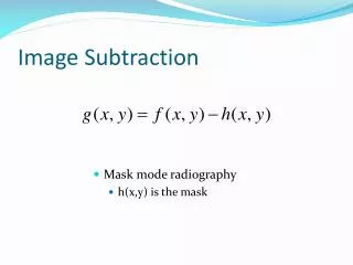
Image Subtraction • Mask mode radiography • h(x,y) is the mask
Image Enhancement in the Spatial Domain
Image Averaging • A noisy image: • Averaging M different noisy images:
Image Averaging • As M increases, the variability of the pixel values at each location decreases. • This means that g(x,y) approaches f(x,y) as the number of noisy images used in the averaging process increases. • Registering of the images is necessary to avoid blurring in the output image.
Image Enhancement in the Spatial Domain
Image Enhancement in the Spatial Domain
Local Enhancement • When it is necessary to enhance details over smaller areas • To devise transformation functions based on the gray-level distribution in the neighborhood of every pixel
Local Enhancement • The procedure is: • Define a square (or rectangular) neighborhood and move the center of this area from pixel to pixel. • At each location, the histogram of the points in the neighborhood is computed and either a histogram equalization or histogram specification transformation function is obtained.
Local Enhancement • More procedure: • This function is finally used to map the gray level of the pixel centered in the neighborhood. • The center is then moved to an adjacent pixel location and the procedure is repeated.
Spatial Filtering • Use of spatial masks for image processing (spatial filters) • Linear and nonlinear filters • Low-pass filters eliminate or attenuate high frequency components in the frequency domain (sharp image details), and result in image blurring.
Spatial Filtering • High-pass filters attenuate or eliminate low-frequency components (resulting in sharpening edges and other sharp details). • Band-pass filters remove selected frequency regions between low and high frequencies (for image restoration, not enhancement).
Spatial Filtering a=(m-1)/2 and b=(n-1)/2, m x n (odd numbers) • For x=0,1,…,M-1 and y=0,1,…,N-1 • Also called convolution (primarily in the frequency domain)
Spatial Filtering • The basic approach is to sum products between the mask coefficients and the intensities of the pixels under the mask at a specific location in the image: (for a 3 x 3 filter)
Image Enhancement in the Spatial Domain
Spatial Filtering • Non-linear filters also use pixel neighborhoods but do not explicitly use coefficients • e.g. noise reduction by median gray-level value computation in the neighborhood of the filter
Smoothing Filters • Used for blurring (removal of small details prior to large object extraction, bridging small gaps in lines) and noise reduction. • Low-pass (smoothing) spatial filtering • Neighborhood averaging - Results in image blurring
Image Enhancement in the Spatial Domain
Image Enhancement in the Spatial Domain
Image Enhancement in the Spatial Domain
Image Enhancement in the Spatial Domain
Smoothing Filters • Median filtering (nonlinear) • Used primarily for noise reduction (eliminates isolated spikes) • The gray level of each pixel is replaced by the median of the gray levels in the neighborhood of that pixel (instead of by the average as before).
Chapter 3 Image Enhancement in the Spatial Domain