An Exact Algorithm for Difficult Detailed Routing Problems
An Exact Algorithm for Difficult Detailed Routing Problems. Kolja Sulimma Wolfgang Kunz J. W.-Goethe Universität Frankfurt. Motivation: routing for automated leaf cell generation. 1-D and 1.5-D cells channel routing seems more adequate than maze routing

An Exact Algorithm for Difficult Detailed Routing Problems
E N D
Presentation Transcript
An Exact Algorithm for Difficult Detailed Routing Problems Kolja Sulimma Wolfgang Kunz J. W.-Goethe Universität Frankfurt
Motivation:routing for automated leaf cell generation • 1-D and 1.5-D cells • channel routing seems more adequate than maze routing • Scenario somewhat different from conventional inter cell channel routing
Motivation:channel routing for automated leaf cell generation • a typical routing channel in a standard cell layout looks like this: • long channel with many tracks
Motivation:channel routing for automated leaf cell generation • a typical routing channel in a standard cell layout looks like this: • long channel with many tracks • fast algorithms like “Greedy Router” perform very well: they need only one or two tracks more than the optimal solution
Motivation:channel routing for automated leaf cell generation • a typical routing channel in a standard cell layout looks like this: • long channel with many tracks • fast algorithms like “Greedy Router” perform very well: they need only one or two tracks more than the optimal solution • some algorithms need a few extra columns
Motivation:channel routing for automated leaf cell generation • a channel in a leaf cell is much smaller
Motivation:channel routing for automated leaf cell generation • a channel in a leaf cell is much smaller • the use of extra area is relatively expensive
Motivation:channel routing for automated leaf cell generation • a channel in a leaf cell is much smaller • the use of extra area is expensive • or might simply be not feasible
Motivationchannel routing for automated leaf cell generation small problem instances: • small constant area overhead of heuristical algorithms becomes a large relative area overhead • asymptotically slow algorithms can be practical • difficult instances • obstacles / keep-out regions • dense terminal placement
Problem Formulationrouting model Grid-based over the cell channel routingin the restricted two layer routing model • grid-based • all elements are aligned to a routing grid • over-the-cell-routing • terminals can be located anywhere in the channel, not only at the top or bottom boundary • restricted two layer model • one layer for horizontal connections (trunks) • one layer for vertical connections (doglegs) • arbitrary obstacles • Each signal crosses each column at most once • (no forks or detours)
Problem Formulationexample channel segment • Connect all terminals that belong to the same net in a channel of length n and a given height of t tracks 1 1 3 5 3 5 2 4 2 1 4
Problem Formulationexample channel segment • Connect all terminals that belong to the same net in a channel of length n and a given height of t tracks 1 1 1 3 5 3 3 5 2 4 2 1 4 4
Algorithmic Approachdecision problem • algorithm does not search for a minimum height routing • tries to find a routing for a given channel height of t tracks • this is all that is needed for constant height leaf cells • minimization is done by iterating over t • obviously increases the runtime • in the paper we show that the overhead is only O(1)
Algorithmic Approachdynamic programming • Sweep over the channel from left to right column by column like the “Greedy Router” • Use track assignments to record for each track the signal that leaves the current column on this track • “Greedy Router” heuristically selects one track assignment for each column • We enumerate all reachable track assignments for the column • Dynamic programming prevents an exponential growth of the search space with the channel length
Algorithmpseudo code for (each column) { for (each possible track assignment m of the previous column) { • check if m valid in this column with respect to terminals and obstacles; use m to generate new track assignments by adding all combinations of doglegs; } }
Algorithmexample • Denote a track assignment by a t-tupel of integers in the range [0, ..., t], where 0 means an empty track • How cancan signals 1 and 2 leave column 5 and enter column 6? 1 1 1 1 3 5 3 3 5 2 2 4 2 1 4 4
Algorithmexample • Denote a track assignment by a t-tupel of integers in the range [0, ..., t], where 0 means an empty track • How cancan signals 1 and 2 leave column 5 and enter column 6? 1 0 2 0 1 1 1 1 1 3 5 3 3 5 2 4 2 2 1 4 4
Algorithmexample • Denote a track assignment by a t-tupel of integers in the range [0, ..., t], where 0 means an empty track • How cancan signals 1 and 2 leave column 5 and enter column 6? 1 0 2 0 0 1 2 0 1 1 1 1 3 5 3 1 3 5 2 4 2 2 1 4 4
Algorithmexample • Denote a track assignment by a t-tupel of integers in the range [0, ..., t], where 0 means an empty track • How cancan signals 1 and 2 leave column 5 and enter column 6? 1 0 2 0 0 1 2 0 0 0 2 1 1 1 1 1 3 5 3 3 5 2 4 2 2 1 1 4 4
Algorithmexample • Denote a track assignment by a t-tupel of integers in the range [0, ..., t], where 0 means an empty track • How cancan signals 1 and 2 leave column 5 and enter column 6? 1 0 2 0 0 1 2 0 0 0 2 1 1 2 0 0 1 1 1 1 1 3 5 3 2 3 5 2 4 2 1 4 4
Algorithmexample • Denote a track assignment by a t-tupel of integers in the range [0, ..., t], where 0 means an empty track • How cancan signals 1 and 2 leave column 5 and enter column 6? 1 0 2 0 0 1 2 0 0 0 2 1 1 2 0 0 1 0 0 2 1 1 1 1 1 3 5 3 3 5 2 4 2 1 2 4 4
Algorithmexample • Denote a track assignment by a t-tupel of integers in the range [0, ..., t], where 0 means an empty track • How cancan signals 1 and 2 leave column 5 and enter column 6? 1 0 2 0 0 1 2 0 0 0 2 1 1 2 0 0 1 0 0 2 0 1 0 2 1 1 1 1 3 5 3 1 3 5 2 4 2 1 2 4 4
Algorithmdetails of column processing // takes as input a set Mi-1 of all track assignments of column i-1 and // produces a set Mi of all track assignments for column i next_column(Mi-1, i) { Mi:= Ø; for (each m Mi-1) { m := removeRightEdgeTerminals(m, i-1); m := addLeftEdgeTerminals(m, i); m := connectTerminals(m, i); m := checkForObstacles(m, i); if (m ≠ 0) { Mi := Mi {m}; Mi := Mi doglegs(m); } } }
removeRightEdgeTerminals()addLeftEdgeTerminals() • Remove all signals that had their last terminal on the previous column. • Add signals to the assignment that have their first terminal on the current column. • Delete assignment if above is impossible
1 4 removeRightEdgeTerminals()addLeftEdgeTerminals() • Remove all signals that had their last terminal on the previous column. • Add signals to the assignment that have their first terminal on the current column. • Delete assignment if above is impossible 1 0 2 0 0 1 2 0 0 0 2 1 1 2 0 0 1 0 0 2 0 1 0 2
1 4 removeRightEdgeTerminals()addLeftEdgeTerminals() • Remove all signals that had their last terminal on the previous column. • Add signals to the assignment that have their first terminal on the current column. • Delete assignment if above is impossible 1 2 4 0 1 0 4 2 0 1 4 2 1 0 2 0 0 1 2 0 0 0 2 1 1 2 0 0 1 0 0 2 0 1 0 2
connectTerminals() • Existing signals might have terminals in this column that are not connected by the incoming assignment. • Add dogleg to connect the signal to the terminal. • Delete the assignment if the track with the terminal is blocked by another signal. 1 2 4 0 1 0 4 2 0 1 4 2 1 2 4 0 1 0 4 2 0 1 4 2 1 1 1 1 4 4 4 4 2 2
doglegs() • Enumerate all the possible dogleg combinations for this assignment. • Multiple layouts might generate the same track assignment. • These layouts are equivalent under routability aspects • only one is selected by dynamic programming • selection can be used to minimize number of vias, wire length, ... 1 0 4 2 1 0 4 2 1 2 4 0 1 0 4 2 1 1 1 1 4 4 4 4 2 2
Computational Complexityworst case • Up to t! possible assignments per column • dogleg() dominates all other subroutines • less than 2t/2 doglegs per assignment • worst case runtime per column O(t!2t) • O(n•t!2t) for a channel of length n • fixed parameter tractable: • overall runtime linear for a fixed channel height • runtime exponential in the channel height
Data StructuresMDDs • Represent the set of track assignments by its characteristic function f:[0, ..., t]t {0, 1} • represent f by an MDD (Multi Valued Decision Diagram) • reduces the size of the representation • typically 1M assignments require 80K MDD-nodes • allows efficient manipulation of the assignments in the set
Track 0 0 0 0 0 0 0 0 0 0 4 4 4 4 4 4 4 4 4 3 3 3 3 3 3 3 3 3 1 1 1 1 1 1 1 1 1 2 2 2 2 2 2 2 2 2 1 0 2 0 0 1 2 0 0 0 2 1 1 2 0 0 1 0 0 2 0 1 0 2 Track 1 Track 2 Track 3 1 Data StructuresMDD example • MDD representation of the example set in column 6 • connections to the 0-terminal are omitted for clarity.
Track 0 0 0 0 0 0 0 0 0 0 4 4 4 4 4 4 4 4 4 3 3 3 3 3 3 3 3 3 1 1 1 1 1 1 1 1 1 2 2 2 2 2 2 2 2 2 Track 1 Track 2 Track 3 Data StructuresMDD example • Each path from the root to the 1-terminal represents a track assignment 1 0 2 0 0 1 2 0 0 0 2 1 1 2 0 0 1 0 0 2 0 1 0 2 1
Track 0 0 0 0 0 0 0 0 0 0 4 4 4 4 4 4 4 4 4 3 3 3 3 3 3 3 3 3 1 1 1 1 1 1 1 1 1 2 2 2 2 2 2 2 2 2 Track 1 Track 2 Track 3 Data StructuresMDD example • Each path from the root to the 1-terminal represents a track assignment 1 0 2 0 0 1 2 0 0 0 2 1 1 2 0 0 1 0 0 2 0 1 0 2 1
Track 0 0 0 0 0 0 0 0 0 0 4 4 4 4 4 4 4 4 4 3 3 3 3 3 3 3 3 3 1 1 1 1 1 1 1 1 1 2 2 2 2 2 2 2 2 2 Track 1 Track 2 Track 3 Data StructuresMDD example • Each path from the root to the 1-terminal represents a track assignment 1 0 2 0 0 1 2 0 0 0 2 1 1 2 0 0 1 0 0 2 0 1 0 2 1
Track 0 0 0 0 0 0 0 0 0 0 4 4 4 4 4 4 4 4 4 3 3 3 3 3 3 3 3 3 1 1 1 1 1 1 1 1 1 2 2 2 2 2 2 2 2 2 Track 1 Track 2 Track 3 Data StructuresMDD example • Each path from the root to the 1-terminal represents a track assignment 1 0 2 0 0 1 2 0 0 0 2 1 1 2 0 0 1 0 0 2 0 1 0 2 1
Track 0 0 0 0 0 0 0 0 0 0 4 4 4 4 4 4 4 4 4 3 3 3 3 3 3 3 3 3 1 1 1 1 1 1 1 1 1 2 2 2 2 2 2 2 2 2 Track 1 Track 2 Track 3 Data StructuresMDD example • Each path from the root to the 1-terminal represents a track assignment 1 0 2 0 0 1 2 0 0 0 2 1 1 2 0 0 1 0 0 2 0 1 0 2 1
Track 0 0 0 0 0 0 0 0 0 0 4 4 4 4 4 4 4 4 4 3 3 3 3 3 3 3 3 3 1 1 1 1 1 1 1 1 1 2 2 2 2 2 2 2 2 2 Track 1 Track 2 Track 3 Data StructuresMDD example • Each path from the root to the 1-terminal represents a track assignment 1 0 2 0 0 1 2 0 0 0 2 1 1 2 0 0 1 0 0 2 0 1 0 2 1
Track 0 0 0 0 0 0 0 0 0 0 4 4 4 4 4 4 4 4 4 1 0 2 0 0 1 2 0 0 0 2 1 1 2 0 0 1 0 0 2 0 1 0 2 3 3 3 3 3 3 3 3 3 1 1 1 1 1 1 1 1 1 2 2 2 2 2 2 2 2 2 Track 1 Track 2 Track 3 Data StructuresMDD example: LeftEdgePorts() • To be able to connect a new signal to track 2 the subset of assignments with an empty track 2 must be found • calculate cofactor f|track2=0 1 4 1
Track 0 0 0 0 0 0 0 0 0 0 4 4 4 4 4 4 4 4 4 1 0 2 0 0 1 2 0 0 0 2 1 1 2 0 0 1 0 0 2 0 1 0 2 3 3 3 3 3 3 3 3 3 1 1 1 1 1 1 1 1 1 2 2 2 2 2 2 2 2 2 Track 1 Track 2 Track 3 Data StructuresMDD example: LeftEdgePorts() • To be able to connect a new signal to track 2 the subset of assignments with an empty track 2 must be found • calculate cofactor f|track2=0 1 4 1
Track 0 0 0 0 0 0 0 0 4 4 4 4 4 4 4 3 3 3 3 3 3 3 1 1 1 1 1 1 1 2 2 2 2 2 2 2 Track 1 Track 2 Track 3 Data StructuresMDD example: LeftEdgePorts() 1 2 0 0 1 0 0 2 0 1 0 2 • To be able to connect a new signal to track 2 the subset of assignments with an empty track 2 must be found • calculate cofactor f|track2=0 1 4 1
Track 0 0 0 0 0 0 0 0 4 4 4 4 4 4 4 3 3 3 3 3 3 3 1 1 1 1 1 1 1 2 2 2 2 2 2 2 Track 1 Track 2 Track 3 Data StructuresMDD example: LeftEdgePorts() 1 2 0 0 1 0 0 2 0 1 0 2 • To insert signal 4 in the empty track move track 2 edges from 0 to 4 1 4 1
Track 0 0 0 0 0 0 0 0 4 4 4 4 4 4 4 3 3 3 3 3 3 3 1 1 1 1 1 1 1 2 2 2 2 2 2 2 Track 1 Track 2 Track 3 Data StructuresMDD example: LeftEdgePorts() 1 2 0 0 1 0 0 2 0 1 0 2 • To insert signal 4 in the empty track move track 2 edges from 0 to 4 1 4 1
Track 0 0 0 0 0 0 0 0 4 4 4 4 4 4 4 3 3 3 3 3 3 3 1 1 1 1 1 1 1 2 2 2 2 2 2 2 Track 1 Track 2 Track 3 Data StructuresMDD example: LeftEdgePorts() 1 2 4 0 1 0 4 2 0 1 4 2 • To insert signal 4 in the empty track move track 2 edges from 0 to 4 1 4 1
Experimental results runtime per column in milliseconds #tracks Hashset MDD 3 2 5 5 4 5 7 100 5 9 6000 20 11 300 13 8000
Conclusion • Intra cell channel routing can be solved exactly by exhaustive enumeration of reachable track assignments • dynamic programming yields a runtime linear in the channel length • Possible application to conventional channel routing: • less than exhaustive search • more than one assignment per column as “Greedy Router” does. • => heuristically select a set of maybe a few hundred track assignments for each column