CPCS 391 Computer Graphics 1

1. CPCS 391 Computer Graphics 1 Instructor: Dr. Sahar Shabanah Lecture 3

2. Scan conversion Algorithms • Primitives and Attributes • Why Scan Conversion? • Algorithms for Scan Conversion: • Lines • Circles • Ellipses • Filling • Polygons

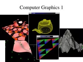
3. Scan Conversion Problem • To represent a perfect image as a bitmapped image.

4. Line Drawing Algorithms • Lines are used a lot - want to get them right. • Lines should appear straight, not jagged. • Horizontal, vertical and diagonal easy, others difficult • Lines should terminate accurately. • Lines should have constant density. • Line density should be independent of line length or angle. • Lines should be drawn rapidly. • Efficient algorithms.

5. (xi,Round(yi+m)) Desired Line (xi,yi) (xi,Round(yi)) (xi,yi +m) DDA: Digital Differential Analyzer • Line: Left to Right: 1- Slope m>0: • sample at unit x intervals ( Δx= 1), • calculate each succeeding y value as

6. DDA • 2- Slope m<0: • sample at unit y intervals ( Δy= 1), • calculate each succeeding x value as • Line: from Right to Left 3- Slope m> 0: 4- Slope m< 0:

7. DDA Advantages Disadvantages • Faster than brute force. • Based on Calculating either ∆x or ∆y. • Mathematically well defined • Floating point • Round off error. • Time consuming arithmetic

8. Bresenhams Line Algorithm • Accurate • Efficient • Integer Calculations • Uses Symmetry for other lines • Adapted to display circles, ellipses and curves • It has been proven that the algorithm gives an optimal fit for lines

9. Bresenhams Line Algorithm yk+1 d2 y d1 yk Xk+1

10. Bresenhams Line Algorithm

11. Bresenhams Line Algorithm • The sign of pk is the same as the sign of d1 – d2, • since Δx> 0 for our example. Parameter c is independent and will be eliminated in the recursive calculations for pk. • If the pixel at yk is closer to the line path than the pixel at yk+l (that is, d1 < d2), then decision parameter pk is negative. In that case, we plot the lower pixel; otherwise, we plot the upper pixel.

12. Bresenhams Line Algorithm This recursive calculation of decision parameters is performed at each integer x position, starting at the left coordinate endpoint of the line. The first parameter, po is evaluated from Eq. 3-12 at the starting pixel position (xo, yo) and with m evaluated as Δy/Δx:

13. Bresenhams Line Drawing Algorithm • Input the two line endpoints, store the left endpoint (x0,y0). • Plot the first point (x0,y0). • Calculate constants ∆x, ∆y, and 2∆y - 2∆x and 2∆y, get starting values for decision parameter pk, p0=2∆y-∆x • At each xk along the line, starting at k = 0, do the following test: if pk < 0, the next point to plot is(xk+1, yk) pk+1 = pk + 2∆y else, the next point to plot is(xk+1, yk+1) pk+1=pk +2∆y-2∆x • Repeat step 4. ∆x times.

14. Bresenhams Line Algorithm

15. Midpoint Line Algorithm If (BlueLine < Midpoint) Plot_East_Pixel(); Else Plot_Northeast_Pixel();

16. Midpoint Line Algorithm • Find an equation, given a line and a point, that will tell us if the point is above or below that line? • If F(x,y) ==0 • (x,y) on the line • <0 for points below the line • >0 for points above the line • d=F(M)

17. Midpoint Line Algorithm • P=(xp, yp) is pixel chosen by the algorithm in previous step • To calculate d incrementally we require dnew • If d > 0 then choose NE Yp+2 MNE NE Yp+1 M yp E P=(xp, yp) xp xp+1 xp+2 Next Current Previous

18. Yp+2 NE Yp+1 M ME yp E P=(xp, yp) xp xp+1 xp+2 Next Previous Current Midpoint Line Algorithm • If d < 0 then choose E

19. Midpoint Line Algorithm • To find Initial value of d NE M E P=(x0, y0) x0 x0+1 Only fractional value Start Initial do • Multiply by 2 to avoid fractions. Redefine d0, E, NE

20. Midpoint Line Algorithm • Midpoint: Looks at which side of the line the mid point falls on. • Bresenham: Looks at sign of scaled difference in errors. • It has been proven that Midpoint is equivalent to Bresenhams for lines.

21. void MidpointLine(int x0, int y0, int x1, int y1, int color) { int dx = x1 – x0, dy = y1 – y0; intd = 2*dy – dx; intdE = 2*dy, dNE = 2*(dy – dx); int x = x0, y = y0; WritePixels(x, y, color); while (x < x1) { if (d <= 0) { // Current d d += dE; // Next d at E x++; } else { d += dNE; // Next d at NE x++; y++ }Write8Pixels(x, y, color);}}

22. Midpoint Circle Algorithm • Implicit of equation of circle is:x2 + y2 - R2 = 0, at origin • Eight way symmetry  require to calculate one octant • For each pixel (x,y), there are 8 symmetric pixels • In each iteration only calculate one pixel, but plot 8 pixels

23. P=(xp, yp) E yp ME M yp – 1 SE MSE yp – 2 xp xp+1 xp+2 Next Current Previous Midpoint Circle Algorithm • Define decision variable d as:

24. P=(xp, yp) E yp ME d < 0 M yp – 1 yp – 2 xp xp+1 xp+2 Next Current Previous Midpoint Circle Algorithm • If d <= 0 then midpoint m is inside circle • we choose E • Increment x • y remains unchanged

25. P=(xp, yp) yp M d > 0 yp – 1 SE MSE yp – 2 xp xp+1 xp+2 Next Current Midpoint Circle Algorithm • If d > 0 then midpoint m is outside circle • we choose E • Increment x • Decrement y Previous

26. Midpoint Circle Algorithm Initial condition • Starting pixel (0, R) • Next Midpoint lies at (1, R – ½) • d0 = F(1, R – ½) = 1 + (R2 – R + ¼) – R2 = 5/4 – R • To remove the fractional value 5/4 : • Consider a new decision variable h as, h = d – ¼ • Substituting d for h + ¼, • d0=5/4 – R h = 1 – R • d < 0 h < – ¼ h < 0 • Since h starts out with an integer value and is incremented by integer value (E or SE), e can change the comparison to just h < 0

27. Midpoint Circle Algorithm voidMidpointCircle(intradius, intvalue) {intx = 0; inty = radius ; intd = 1 – radius ; CirclePoints(x, y, value); while (y > x) { if (d < 0) { /* Select E */ d += 2 * x + 3; } else { /* Select SE */ d += 2 * ( x – y ) + 5; y– –; } x++; CirclePoints(x, y, value); } }

28. Midpoint Circle Algorithm Void CirclePoints(intx,inty, float value) { SetPixel(x,y); SetPixel(x,-y); SetPixel(-x,y); SetPixel(-x,-y); SetPixel(y,x); SetPixel(y,-x); SetPixel(-y,x); SetPixel(-y,-x); }

29. Midpoint Circle Algorithm • Second-order differences can be used to enhance performance. E M SE MSE E is chosen SE is chosen

30. Midpoint Circle Algorithm voidMidpointCircle(intradius, intvalue) {intx = 0; inty = radius ; intd = 1 – radius ; intdE = 3; intdSE = -2*radius+5; CirclePoints(x, y, value); while (y > x) { if (d < 0) {/* Select E */ d += dE; dE += 2; dSE += 2; } else { /* Select SE */ d += dSE; dE += 2; dSE += 4; y– –;} x++; CirclePoints(x, y, value);} }

31. (-x1,y1) (x1,y1) (-x2,y2) (x2,y2) (-x2,-y2) (x2,-y2) (-x1,-y1) (x1,-y1) Midpoint Ellipse Algorithm • Implicit equation is: F(x,y) = b2x2 + a2y2 – a2b2 = 0 • We have only 4-way symmetry • There exists two regions • In Region 1dx > dy • Increase x at each step • y may decrease • In Region 2dx < dy • Decrease y at each step • x may increase

32. Tangent Slope = -1 E Gradient Vector SE Region 1 Region 2 SE S Midpoint Ellipse Algorithm

33. P=(xp, yp) E yp ME M yp – 1 SE MSE yp – 2 xp xp+1 xp+2 Next Current Previous Midpoint Ellipse Algorithm • In region 1

34. Previous Current Next xp xp+1 xp+2 P=(xp, yp) yp yp – 1 SE S M yp – 2 MS MSE Midpoint Ellipse Algorithm • In region 2

35. Midpoint Ellipse Algorithm DPx=2*ry*ry; Dpy=2*rx*rx; x=0; y=ry; Px=0; Py=2*rx*rx*ry; f=ry*ry +rx*rx(0.25-ry ); ry2=ry *ry; Set4Pixel(x,y); while (px<py ) //Region I { x=x+1; Px=Px+DPx; if (f>0) // Bottom case {y=y -1; Py=Py -Dpy ; f=f+ry2+Px-Py;} else // Top case f=f+ry2+Px; Set4Pixel(x,y);