Download
1 / 1

E N D
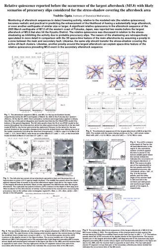
Monitoring of aftershock sequences to detect lowering activity, relative to the modeled rate (the relative quiescence), becomes realistic and practical in predicting the enhancement of the likelihood of having a substantially large aftershock, or even another earthquake of similar size or larger. A significant relative quiescence in the aftershock sequence of the 2005 March earthquake of M7.0 off the western coast of Fukuoka, Japan, was reported two weeks before the largest aftershock of M5.8 that also hit the Kyushu District. The relative quiescence was discussed in relation to the stress-shadowing as inhibiting the activity due to probable precursory slips. The reason of the shadowing are retrospectively speculated in more detail in comparison with the 3D space-time feature of the main aftershocks by assuming a preslip in a zone between the main and secondary fault. Likewise, the same slip should transfer the stress-shadow covering the active off-fault clusters. Likewise, another preslip around the largest aftershock can explain space-time feature of the relative quiescence preceding M5.0 event in the secondary aftershock sequence. Relative quiescence reported before the occurrence of the largest aftershock (M5.8) with likely scenarios of precursory slips considered for the stress-shadow covering the aftershock area Fig. 1. The aftershock sequence (M2.6+ and M3+ for the top and bottom blocks, respectively) led by the M7.0 earthquake of March 20, 2005 in the Fukuoka-Ken western offshore, till the April 4, 2005: their cumulative numbers and magnitudes against ordinary time (the top of the paired diagrams) and transformed time by the fitted ETAS model (the bottom of the paired diagrams). The left side panels show the fit of one ETAS model to the events throughout the entire period, while the other panels show the best fit of the two-fold model (ETAS for the former period and the stationary Poisson for the latter) for the two periods divided at the possible change-points (vertical dotted lines) even taking account of the model complexity including the searched change-point.: in M2.6+ case it is at March 28 (AIC = - 5.2), and in M3.0+ case those are either March 27 (AIC = - 4.2), or the three-fold model divided at March 21 and then 27 (AIC = - 4.2). Fig. 2. The aftershock sequences till the largest aftershock of M5.8 at April 20, 2005. The models with the same change-points as in Fig. 1 still remain better fitted with AIC = 0.0 for M2.6+ case and AIC = - 7.8 for M3.0+ case. Yosihiko Ogata, Institute of Statistical Mathematics Fig. 4. The CFS contours at the depth of 7km for the off-fault aftershocks in the region A, the cumulative number of which against the time is shown in the bottom middle panel where the vertical dotted line indicates the occurrence of the largest aftershock of M5.8. The source models are of the mainshock5) in the top panels and of the assumed precursory slip(left lateral, strike = 320 , cf. Fig. 3)in the bottom panels; and the strike angle of the receiver fault is 300 and 320 in the northern part (left panel) and southern part (right panel) of the region A, respectively. Fig. 3. The left-side two panels show aftershock epicenters (top) and the projection of hypocenters to plane of X-Y against depth (bottom). The middle two panels show the depth against elapsed time of events in the entire aftershock region (top) and in the region close to the largest aftershock (bottom). Black circles represent the aftershocks after the largest aftershock. The right-side two panels indicate CFS contours at the depth of 5km (top) and 10km (bottom) for the aftershocks of similar mechanism5) to the mainshock’s assuming the precursory slip on the yellow color rectangular region(H = 8km, L = W = 8km,strike = 320 )shown in the left panels. Fig. 6. The secondary aftershock sequences of the largest aftershock of M5.8 till the M5.0 event at May 2, 2005. The significance of the change-point models against the normal decay by fitting the modified Omori model (red curves) is AIC = - 1.0. The bottom panels show the CFS contours at the depths shown in the figure bottom. The source models are of the largest aftershock (M5.8, left diagram) and of the assumed slip (right diagram) preceding M5.0 events whose depth and mechanisms indicated in the figure are due to the JMA; and the receiver fault is opposite to each other. The top right panel shows XY segment versus time plot of the secondary aftershocks where dotted line indicates the occurrence time of the M5 event. Fig. 5. The secondary aftershock sequences of the largest aftershock of M5.8 till the M5.0 event at May 2, 2005. The significance of the change-point models against the normal decay by fitting the modified Omori model (red curves) is AIC = - 1.0. The bottom panels show the CFS contours at the depths shown in the figure bottom. The source models are of the largest aftershock (M5.8, left diagram) and of the assumed slip (right diagram) preceding M5.0 events whose depth and mechanisms indicated in the figure are due to the JMA; and the receiver fault is opposite to each other. The top right panel shows XY segment versus time plot of the secondary aftershocks where dotted line indicates the occurrence time of the M5 event.