6.094 Introduction to programming in MATLAB

6.094Introduction to programming in MATLAB Lecture 2: Visualization and Programming Danilo Šćepanović IAP 2010

Homework 1 Recap • How long did it take to do required problems? • Did anyone do optional problems? • Was level of guidance appropriate? • Unanswered Questions? • Some things that came up: • Use of semicolon – never required if one command per line. You can also put multiple commands on one line; in this case a semicolon is necessary to separate commands: • x=1:10; y=(x-5).^2; plot(x,y); • Assignment using indices – remember that you can index into matrices to either look up values or to assign value: • x=rand(50,1); inds=find(x<0.1); y=x(inds); x(inds)=-x(inds); x(inds)=3;

Outline • Functions • Flow Control • Line Plots • Image/Surface Plots • Vectorization

Help file Function declaration Outputs Inputs User-defined Functions • Functions look exactly like scripts, but for ONE difference • Functions must have a function declaration

Inputs must be specified function [x, y, z] = funName(in1, in2) Must have the reserved word: function Function name should match m-file name If more than one output, must be in brackets User-defined Functions • Some comments about the function declaration • No need for return: Matlab 'returns' the variables whose names match those in the function declaration • Variable scope: Any variables created within the function but not returned disappear after the function stops running

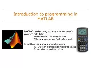
Functions: overloading We're familiar with zeros size length sum Look at the help file for size by typing help size The help file describes several ways to invoke the function D = SIZE(X) [M,N] = SIZE(X) [M1,M2,M3,...,MN] = SIZE(X) M = SIZE(X,DIM)

Functions: overloading Matlab functions are generally overloaded Can take a variable number of inputs Can return a variable number of outputs What would the following commands return: a=zeros(2,4,8); %n-dimensional matrices are OK D=size(a) [m,n]=size(a) [x,y,z]=size(a) m2=size(a,2) You can overload your own functions by having variable input and output arguments (see varargin, nargin, varargout, nargout)

Functions: Excercise • Write a function with the following declaration:function plotSin(f1) • In the function, plot a sin wave with frequency f1, on the range [0,2π]: • To get good sampling, use 16 points per period.

Functions: Excercise • Write a function with the following declaration:function plotSin(f1) • In the function, plot a sin wave with frequency f1, on the range [0,2π]: • To get good sampling, use 16 points per period. • In an m-file saved as plotSin.m, write the following: • function plotSin(f1)x=linspace(0,2*pi,f1*16+1);figureplot(x,sin(f1*x))

Relational Operators • Matlab uses mostly standard relational operators • equal == • not equal ~= • greater than > • less than < • greater or equal >= • less or equal <= • Logical operators elementwise short-circuit (scalars) • And & && • Or | || • Not~ • Xor xor • All true all • Any true any • Boolean values: zero is false, nonzero is true • See help . for a detailed list of operators

if/else/elseif • Basic flow-control, common to all languages • Matlab syntax is somewhat unique IF if cond commands end ELSE if cond commands1 else commands2 end ELSEIF if cond1 commands1 elseif cond2 commands2 else commands3 end Conditional statement: evaluates to true or false • No need for parentheses: command blocks are between reserved words

for • for loops: use for a known number of iterations • MATLAB syntax: for n=1:100 commands end • The loop variable • Is defined as a vector • Is a scalar within the command block • Does not have to have consecutive values (but it's usually cleaner if they're consecutive) • The command block • Anything between the for line and the end Loop variable Command block

while • The while is like a more general for loop: • Don't need to know number of iterations • The command block will execute while the conditional expression is true • Beware of infinite loops! WHILE while cond commands end

Exercise: Conditionals • Modify your plotSin(f1) function to take two inputs: plotSin(f1,f2) • If the number of input arguments is 1, execute the plot command you wrote before. Otherwise, display the line 'Two inputs were given' • Hint: the number of input arguments are in the built-in variable nargin

Exercise: Conditionals • Modify your plotSin(f1) function to take two inputs: plotSin(f1,f2) • If the number of input arguments is 1, execute the plot command you wrote before. Otherwise, display the line 'Two inputs were given' • Hint: the number of input arguments are in the built-in variable nargin • function plotSin(f1,f2)x=linspace(0,2*pi,f1*16+1);figureif nargin == 1 plot(x,sin(f1*x));elseif nargin == 2 disp('Two inputs were given');end

Plot Options • Can change the line color, marker style, and line style by adding a string argument • plot(x,y,’k.-’); • Can plot without connecting the dots by omitting line style argument • plot(x,y,’.’) • Look at help plot for a full list of colors, markers, and linestyles color marker line-style

Playing with the Plot to select lines and delete or change properties to see all plot tools at once to slide the plot around to zoom in/out

Line and Marker Options • Everything on a line can be customized • plot(x,y,'--s','LineWidth',2,... 'Color', [1 0 0], ... 'MarkerEdgeColor','k',... 'MarkerFaceColor','g',... 'MarkerSize',10) • See doc line_props for a full list of properties that can be specified You can set colors by using a vector of [R G B] values or a predefined color character like 'g', 'k', etc.

Cartesian Plots • We have already seen the plot function • x=-pi:pi/100:pi; • y=cos(4*x).*sin(10*x).*exp(-abs(x)); • plot(x,y,'k-'); • The same syntax applies for semilog and loglog plots • semilogx(x,y,'k'); • semilogy(y,'r.-'); • loglog(x,y); • For example: • x=0:100; • semilogy(x,exp(x),'k.-');

3D Line Plots • We can plot in 3 dimensions just as easily as in 2 • time=0:0.001:4*pi; • x=sin(time); • y=cos(time); • z=time; • plot3(x,y,z,'k','LineWidth',2); • zlabel('Time'); • Use tools on figure to rotate it • Can set limits on all 3 axes • xlim, ylim, zlim

Axis Modes • Built-in axis modes • axis square • makes the current axis look like a box • axis tight • fits axes to data • axis equal • makes x and y scales the same • axis xy • puts the origin in the bottom left corner (default for plots) • axis ij • puts the origin in the top left corner (default for matrices/images)

Multiple Plots in one Figure • To have multiple axes in one figure • subplot(2,3,1) • makes a figure with 2 rows and three columns of axes, and activates the first axis for plotting • each axis can have labels, a legend, and a title • subplot(2,3,4:6) • activating a range of axes fuses them into one • To close existing figures • close([1 3]) • closes figures 1 and 3 • close all • closes all figures (useful in scripts/functions)

Copy/Paste Figures Figures can be pasted into other apps (word, ppt, etc) Edit copy options figure copy template Change font sizes, line properties; presets for word and ppt Edit copy figure to copy figure Paste into document of interest

Saving Figures • Figures can be saved in many formats. The common ones are: .fig preserves all information .bmp uncompressed image .eps high-quality scaleable format .pdf compressed image

Advanced Plotting: Exercise • Modify the plot command in your plotSin function to use squares as markers and a dashedred line of thickness 2 as the line. Set the marker face color to be black (properties are LineWidth, MarkerFaceColor) • If there are 2 inputs, open a new figure with 2 axes, one on top of the other (not side by side), and activate the top one (subplot) plotSin(6) plotSin(1,2)

Advanced Plotting: Exercise • Modify the plot command in your plotSin function to use squares as markers and a dashedred line of thickness 2 as the line. Set the marker face color to be black (properties are LineWidth, MarkerFaceColor) • If there are 2 inputs, open a new figure with 2 axes, one on top of the other (not side by side), and activate the top one (subplot) • if nargin == 1 plot(x,sin(f1*x),'rs--',... 'LineWidth',2,'MarkerFaceColor','k');elseif nargin == 2 subplot(2,1,1);end

Visualizing matrices • Any matrix can be visualized as an image • mat=reshape(1:10000,100,100); • imagesc(mat); • colorbar • imagesc automatically scales the values to span the entire colormap • Can set limits for the color axis (analogous to xlim, ylim) • caxis([3000 7000])

Colormaps • You can change the colormap: • imagesc(mat) • default map is jet • colormap(gray) • colormap(cool) • colormap(hot(256)) • See help hot for a list • Can define custom colormap • map=zeros(256,3); • map(:,2)=(0:255)/255; • colormap(map);

Surface Plots • It is more common to visualize surfaces in 3D • Example: • surf puts vertices at specified points in space x,y,z, andconnects all the vertices to make a surface • The vertices can be denoted by matrices X,Y,Z • How can we make these matrices • loop (DUMB) • built-in function: meshgrid

surf • Make the x and y vectors • x=-pi:0.1:pi; • y=-pi:0.1:pi; • Use meshgrid to make matrices (this is the same as loop) • [X,Y]=meshgrid(x,y); • To get function values, evaluate the matrices • Z =sin(X).*cos(Y); • Plot the surface • surf(X,Y,Z) • surf(x,y,Z);

surf Options • See help surf for more options • There are three types of surface shading • shading faceted • shading flat • shading interp • You can change colormaps • colormap(gray)

contour • You can make surfaces two-dimensional by using contour • contour(X,Y,Z,'LineWidth',2) • takes same arguments as surf • color indicates height • can modify linestyle properties • can set colormap • hold on • mesh(X,Y,Z)

Exercise: 3-D Plots • Modify plotSin to do the following: • If two inputs are given, evaluate the following function: • y should be just like x, but using f2. (use meshgrid to get the X and Y matrices) • In the top axis of your subplot, display an image of the Z matrix. Display the colorbar and use a hotcolormap. Set the axis to xy (imagesc, colormap, colorbar, axis) • In the bottom axis of the subplot, plot the 3-D surface of Z (surf)

Exercise: 3-D Plots • function plotSin(f1,f2)x=linspace(0,2*pi,round(16*f1)+1);figureif nargin == 1 plot(x,sin(f1*x),'rs--',... 'LineWidth',2,'MarkerFaceColor','k');elseif nargin == 2 y=linspace(0,2*pi,round(16*f2)+1); [X,Y]=meshgrid(x,y); Z=sin(f1*X)+sin(f2*Y); subplot(2,1,1); imagesc(x,y,Z); colorbar; axis xy; colormap hot subplot(2,1,2); surf(X,Y,Z);end

Exercise: 3-D Plots plotSin(3,4) generates this figure

Specialized Plotting Functions • Matlab has a lot of specialized plotting functions • polar-to make polar plots • polar(0:0.01:2*pi,cos((0:0.01:2*pi)*2)) • bar-to make bar graphs • bar(1:10,rand(1,10)); • quiver-to add velocity vectors to a plot • [X,Y]=meshgrid(1:10,1:10); • quiver(X,Y,rand(10),rand(10)); • stairs-plot piecewise constant functions • stairs(1:10,rand(1,10)); • fill-draws and fills a polygon with specified vertices • fill([0 1 0.5],[0 0 1],'r'); • see help on these functions for syntax • doc specgraph – for a complete list

Revisiting find • find is a very important function • Returns indices of nonzero values • Can simplify code and help avoid loops • Basic syntax: index=find(cond) • x=rand(1,100); • inds = find(x>0.4 & x<0.6); • inds will contain the indices at which x has values between 0.4 and 0.6. This is what happens: • x>0.4 returns a vector with 1 where true and 0 where false • x<0.6 returns a similar vector • The & combines the two vectors using an and • The find returns the indices of the 1's

Example: Avoiding Loops • Given x= sin(linspace(0,10*pi,100)), how many of the entries are positive? Using a loop and if/else count=0; for n=1:length(x) if x(n)>0 count=count+1; end end Being more clever count=length(find(x>0)); • Avoid loops! • Built-in functions will make it faster to write and execute

Efficient Code • Avoid loops • This is referred to as vectorization • Vectorized code is more efficient for Matlab • Use indexing and matrix operations to avoid loops • For example, to sum up every two consecutive terms: • a=rand(1,100); • b=zeros(1,100); • for n=1:100 • if n==1 • b(n)=a(n); • else • b(n)=a(n-1)+a(n); • end • end • Slow and complicated • a=rand(1,100); • b=[0 a(1:end-1)]+a; • Efficient and clean. Can also do this using conv

End of Lecture 2 • Functions • Flow Control • Line Plots • Image/Surface Plots • Vectorization Vectorization makes coding fun!

6.094 Introduction to programming in MATLAB