Excess Rainfall
Excess Rainfall. Reading for today’s material: Sections 5.3-5.7. Slides prepared by V.M. Merwade. Excess rainfall. Rainfall that is neither retained on the land surface nor infiltrated into the soil Graph of excess rainfall versus time is called excess rainfall hyetograph

Excess Rainfall
E N D
Presentation Transcript
Excess Rainfall Reading for today’s material: Sections 5.3-5.7 Slides prepared by V.M. Merwade
Excess rainfall • Rainfall that is neither retained on the land surface nor infiltrated into the soil • Graph of excess rainfall versus time is called excess rainfall hyetograph • Direct runoff = observed streamflow - baseflow • Excess rainfall = observed rainfall - abstractions • Abstractions/losses – difference between total rainfall hyetograph and excess rainfall hyetograph
f-index • f-index: Constant rate of abstraction yielding excess rainfall hyetograph with depth equal to depth of direct runoff • Used to compute excess rainfall hyetograph when observed rainfall and streamflow data are available
f-index method • Goal: pick Dt, and adjust value of M to satisfy the equation • Steps • Estimate baseflow • DRH = streamflow hydrograph – baseflow • Compute rd, rd = Vd/watershed area • Adjust M until you get a satisfactory value of f • ERH = Rm - fDt
Example Have precipitation and streamflow data, need to estimate losses Time Observed Rain Flow in cfs 8:30 203 9:00 0.15 246 9:30 0.26 283 10:00 1.33 828 10:30 2.2 2323 11:00 0.2 5697 11:30 0.09 9531 12:00 11025 12:30 8234 1:00 4321 1:30 2246 2:00 1802 2:30 1230 3:00 713 3:30 394 4:00 354 4:30 303 No direct runoff until after 9:30 And little precip after 11:00 Basin area A = 7.03 mi2
Example (Cont.) • Estimate baseflow (straight line method) • Constant = 400 cfs baseflow
Example (Cont.) • Calculate Direct Runoff Hydrograph • Subtract 400 cfs Total = 43,550 cfs
Example (Cont.) • Compute volume of direct runoff • Compute depth of direct runoff
Example (Cont.) • Neglect all precipitation intervals that occur before the onset of direct runoff (before 9:30) • Select Rm as the precipitation values in the 1.5 hour period from 10:00 – 11:30
Example (Cont.) fDt=0.27
Precipitation Time SCS method • Soil conservation service (SCS) method is an experimentally derived method to determine rainfall excess using information about soils, vegetative cover, hydrologic condition and antecedent moisture conditions • The method is based on the simple relationship that Pe = P - Fa – Ia Pe is runoff volume, P is precipitation volume, Fa is continuing abstraction, and Ia is the sum of initial losses (depression storage, interception, ET)
Precipitation Time Abstractions – SCS Method • In general • After runoff begins • Potential runoff • SCS Assumption • Combining SCS assumption with P=Pe+Ia+Fa
SCS Method (Cont.) • Surface • Impervious: CN = 100 • Natural: CN < 100 • Experiments showed • So
SCS Method (Cont.) • S and CN depend on antecedent rainfall conditions • Normal conditions, AMC(II) • Dry conditions, AMC(I) • Wet conditions, AMC(III)
SCS Method (Cont.) • SCS Curve Numbers depend on soil conditions
Example - SCS Method - 1 • Rainfall: 5 in. • Area: 1000-ac • Soils: • Class B: 50% • Class C: 50% • Antecedent moisture: AMC(II) • Land use • Residential • 40% with 30% impervious cover • 12% with 65% impervious cover • Paved roads: 18% with curbs and storm sewers • Open land: 16% • 50% fair grass cover • 50% good grass cover • Parking lots, etc.: 14%
Example (SCS Method – 1, Cont.) CN values come from Table 5.5.2
Example (SCS Method – 1 Cont.) • Average AMC • Wet AMC
Example (SCS Method – 2) • Given P, CN = 80, AMC(II) • Find: Cumulative abstractions and excess rainfall hyetograph
Example (SCS Method – 2) • Calculate storage • Calculate initial abstraction • Initial abstraction removes • 0.2 in. in 1st period (all the precip) • 0.3 in. in the 2nd period (only part of the precip) • Calculate continuing abstraction
Example (SCS method – 2) • Cumulative abstractions can now be calculated
Example (SCS method – 2) • Cumulative excess rainfall can now be calculated • Excess Rainfall Hyetograph can be calculated
Example (SCS method – 2) • Cumulative excess rainfall can now be calculated • Excess Rainfall Hyetograph can be calculated
Time of Concentration • Different areas of a watershed contribute to runoff at different times after precipitation begins • Time of concentration • Time at which all parts of the watershed begin contributing to the runoff from the basin • Time of flow from the farthest point in the watershed Isochrones: boundaries of contributing areas with equal time of flow to the watershed outlet
Stream ordering • Quantitative way of studying streams. Developed by Horton and then modified by Strahler. • Each headwater stream is designated as first order stream • When two first order stream combine, they produce second order stream • Only when two streams of the same order combine, the stream order increases by one • When a lower order stream combines with a higher order stream, the higher order is retained in the combined stream