Download
1 / 96
970 likes | 1.02k Vues
Detailed theoretical overview of the GS fog/low stratus algorithm for aviation, including fog/cloud definitions, development strategy, and sensor inputs. Discusses algorithm objectives and development approach.

E N D
Algorithm Theoretical Basis (Fog/Low Stratus)Presented byMichael Pavolonis Aviation Application Team STAR With significant contributions from: Corey Calvert (UW/CIMSS)
Algorithm Theoretical Basis • Purpose: Provide product developers, reviewers and users with a theoretical description (scientific and mathematical) of the enterprise GS Fog/Low Stratus algorithm • Will be documented in the ATBD of enterprise GS Fog/Low Stratus products
CDR Requirements Low Cloud and Fog C – CONUS FD – FullDisk M - Mesoscale
CDR Requirements Low Cloud and Fog C – CONUS FD – FullDisk M - Mesoscale
Algorithm Development - Development Strategy • Aviation based fog/low cloud definition • Visual flight rules • ceiling > 3000 ft and/or surface visibility > 5 sm • Marginal visual flight rules • 1000 ft < ceiling < 3000 ft and/or 3 sm < sfc vis < 5 sm • Instrument flight rules • 500 ft < ceiling < 1000 ft and/or 1 sm < sfc vis < 3 sm • Low instrument flight rules • ceiling < 500 ft and/or sfc vis < 1 sm
Algorithm Development - Development Strategy • Aviation based fog/low cloud definition • Visual flight rules • ceiling > 3000 ft and/or surface visibility > 5 sm • Marginal visual flight rules • 1000 ft < ceiling < 3000 ft and/or 3 sm < sfc vis < 5 sm • Instrument flight rules • 500 ft < ceiling < 1000 ft and/or 1 sm < sfc vis < 3 sm • Low instrument flight rules • ceiling < 500 ft and/or sfc vis < 1 sm
ADR Algorithm • There was no ADR performed for the Enterprise GS fog/low stratus products • However, an algorithm was developed to detect fog/low stratus under the GOES-R Future Capabilities project and has already gone through a CDR and TRR • This algorithm was created to mitigate several issues seen in the current 3.9-11μm BTD product currently in operations • Issues with the 3.9-11μm BTD products • Method only designed for nighttime conditions. • False alarms over barren surfaces. • Non-hazardous water clouds are often detected as fog/low cloud • Thresholds and empirical relationship depends on exact sensor characteristics.
CDR Algorithm • Given that the F&PS requires fog/low stratus products to be produced during the day and night, our preferred solution is to utilize the algorithm developed under the GOES-R Future Capabilities project.
Algorithm Objectives • Meet the F&PS requirements for low cloud and fog. • Provide needed performance information to allow for proper use of our products.
Low Cloud and Fog Sensor Inputs Current Input Expected Added Input Possible Added Input
Fog and Low Cloud InputSensor Input Details Possible Added Input GOES-R ABI Low Cloud/Fog requires the following for each pixel: • Calibrated/Navigated ABI brightness temperatures/radiances/reflectances • Spectral response information • Solar-view geometry (satellite zenith, relative azimuth, solar zenith) • Geolocation (latitude, longitude)
Sensor Inputs Channels used in low cloud/fog algorithm
Fog and Low Cloud InputAncillary Input Details • Non-ABI Static Data
Fog and Low Cloud Algorithm InputAncillary Input Details • Non-ABI Dynamic Data
Fog and Low Cloud AlgorithmProduct Precedence Details • Products required to run algorithm
ABI Proxy Data for Fog/Low Cloud AWG Products • Geostationary satellite datasets are used as ABI proxies in algorithm verification/validation • GOES N-P Imagers • Moderate Resolution Imaging Spectroradiometer (MODIS) The data from GOES is considered as a good proxy of ABI since • noise levels are close to expected ABI channels • in geostationary orbit covering the same geographic area as the ABI • Spatial resolution (4 km) somewhat similar to ABI (2 km) • Co-located with high quality ground truth The data from MODIS is considered as a good proxy of ABI since • Spatial resolution (1 km) somewhat similar to ABI (2 km)
ABI Proxy Data Used Current Input Expected Added Input Possible Added Input
Retrieval Strategy (Naïve Bayesian Approach) NWP Static Ancillary Data Daily SST Data + + + -Minimum channel requirement: 0.65, 3.9, 6.7/7.3, 11, and 12/13.3 μm -Previous image for temporal continuity (GEO only) -Cloud Phase -Surface Temperature -Profiles of T and q -RUC/RAP (2-3 hr forecast) or GFS (12 hr forecast) -DEM -Surface Type -Surface Emissivity 0.25 degree OISST Clear Sky RTM NWP RH Profiles IFR Probability Naïve Bayesian Model -RUC/RAP (2-3 hr forecast) or GFS (12 hr forecast) ***IMPORTANT: Other sources of relevant data (e.g. sfc obs) influence results through the model fields
Retrieval Strategy (Naïve Bayesian Approach) Naïve Bayesian Model probability an event occurs given a set of measured features Calculated climatology of event probability an event occurs given no measured features probability an event does not occur given no measured features Conditional probability a set of features are observed given an event occurs Trained using known data Conditional probability a set of features are observed given an event occurs
Retrieval Strategy (single layer liquid fog detection) • The ABI cloud phase/type product is used to identify liquid water clouds • For single layer liquid fog detection, the following physical properties are exploited: • Since the top of fog/low stratus layers is often close to the ground, the temperature difference between the cloud and the surface temperature is typically small. • Since fog/low stratus is not formed by adiabatic cooling brought about by spatially varying vertical motions, it tends to be horizontally uniform in albedo (e.g. reflectivity). • Fog/low clouds are generally composed of small liquid droplets • Fog/low clouds form in environments at or near saturation • Thus, the difference between the observed and clear sky surface temperature, the 3.9 micron reflectance and pseudo-emissivity, the standard deviation of reflectance in a 3 x 3 pixel array and low level moisture are used as fog detection metrics. The strength of the radiometric signal is also taken into account (via a cloud - clear reflectance difference or the 3.9/11 m nighttime signal). • As opposed to using specific fog/no fog thresholds, a training data set is used to assign a fog probability to each non-ice cloud pixel. • This approach does not rely on thresholds or metrics that are highly sensitive to the exact sensor characteristics, so it should not need to be extensively tuned when applied to actual ABI data.
Retrieval Strategy (IFR detection when multi-layered or ice clouds are present) • The ABI cloud phase/type product is used to identify ice clouds, including multilayered ice clouds. • When multi-layered or ice clouds are present, the following physical property is exploited: • Ice clouds, including multi-layered clouds, tend to be elevated and can obscure lower clouds and fog from a satellite point of view • Fog/low clouds beneath ice clouds form in environments at or near saturation • Precipitation from convective clouds can create IFR conditions at or near the surface • Satellites can not see through multiple cloud layers so if the fog/low cloud layer is not the highest cloud layer then it’s spectral information is not seen. • For this reason, only the low level RH information from NWP models is used to detect IFR conditions. • As opposed to using specific fog/no fog thresholds, a training data set is used to assign a fog probability to each multi-layered or ice pixel. • This approach does not rely on thresholds or metrics that are highly sensitive to the exact sensor characteristics, so it should not need to be extensively tuned when applied to actual ABI data.
Retrieval Strategy (IFR detection in the terminator region) • At high daytime solar zenith angles accurate satellite data can be difficult to obtain due to scattering issues • The characteristics of fog/low stratus clouds usually do not drastically change in time so temporal data is used until accurate data is available at lower sun angles • A maximum of 2 scenes within 1 hr of the processed scene are used to temporarily fill gaps in the terminator region • Day-to-night transition • Temporal 3.9 m reflectance and the 0.65 m spatial uniformity metric are used for solar angles between 80-90° • Night-to-day transition • Temporal 3.9 m pseudo-emissivity data is used for solar angles between 85-90° • The NWP data is not dependent on solar angles so the modeled RH and sfc temperature bias are used for all pixels. • Cloud masking can also be difficult in the terminator region so a temporal cloud check is used for sun angles between 70-90°to re-classify ‘clear’ pixels as cloudy when fog/low stratus might be present • This approach does not rely on thresholds or metrics that are highly sensitive to the exact sensor characteristics, so it should not need to be extensively tuned when applied to actual ABI data.
Retrieval Strategy (fog depth) • The fog depth retrieval is performed on all pixels not characterized as ice from the cloud type algorithm • During the day, the fog depth is computed using the retrieved liquid water path and an assumed liquid water content consistent with in-situ measurements of fog. • At night, aregression relationship, conceptually similar to the one developed by Ellrod, is used. • Fog depth retrievals are not possible in the day/night terminator.
Retrieval Strategy (Fog/Low Cloud Detection) • The enterprise GS fog/low cloud detection algorithm can be broken into ????? separate steps. • Using the cloud mask and cloud type/phase results to differentiate water from ice clouds, compute fog detection metrics for all pixels at night and cloudy pixels during the day • Based on the metrics, determine the fog/low cloud probability for each pixel using previously constructed fog probability look-up tables. • ?????
Retrieval Strategy (Fog/Low Cloud Detection) • The enterprise GS fog/low cloud detection algorithm can be broken into 4 separate steps. • Using the cloud mask and cloud type/phase results to differentiate water from ice clouds, compute fog detection metrics for all pixels at night and cloudy pixels during the day • Based on the metrics, determine the fog/low cloud probability for each pixel using previously constructed fog probability look-up tables. • ?????
Cloud Type/Phase Product Full disk cloud type results Water, Supercooled Water, Mixed Phase, Thick Ice, Thin Ice, Multilayered
Physical Description Metric 1: Difference between the radiometrically derived surface temperature and the NWP surface temperature [Day and Night] • For cloudy scenes, the radiometric surface temperature tends to be much lower than the SST or LST given by NWP, unless fog/low cloud is present. In which case, the difference is smaller. • The radiometric surface temperature can be derived from the 11-m radiance by re-arranging the infrared radiative transfer equation. • Note that if one were to use the difference between the observed 11-m brightness temperature and the surface temperature, the results will be sensitive to the water vapor loading, view angle, and sensor characteristics. • The radiometric surface temperature is derived as follows:
Physical Description Metric 1: Difference between the radiometrically derived surface temperature and the NWP surface temperature [Day and Night] Assuming clear conditions : wavelength (11-m in this case) R(): observed radiance Rsfc(): surface radiance Tatm(): total atmospheric transmittance Ratm(): atmospheric radiance sfc(): surface emissivity B-1( ): inverse Planck Function Tsfc: radiometric surface temperature Tnwp: surface temperature from NWP Tsfc_bias: the difference between the radiometric and NWP surface temperatures
Physical Description Full disk view of “surface temperature bias”
Physical Description Full disk view of “surface temperature bias” Low clouds Elevated clouds
Physical Description Metric 2: Low-level Relative Humidity [Day and night] • Fog/low clouds form in environments at or near saturation • low-level RH information is determined using the surface RH and RH profile data from NWP models (RAP/GFS) • The vertical ceiling requirement for fog/low clouds is 1000 ft so the maximum RH from the surface up to 1000 ft above ground level (AGL) is used as the RH metric
Physical Description Full disk view of Max RH in lowest 1000 ft layer AGL Most low-level air at/near saturation Dry low-level air
Physical Description Metric 3: Spatial uniformity at the cloud LRC [Day only] • As stated earlier, fog/low cloud tends to be spatially uniform in albedo. • Consider the standard deviation of a given parameter over a 3 x 3 pixel window. • The standard deviation of the visible reflectance is a useful indicator of fog during the day. • Issues arise near cloud edges where the standard deviations in the visible reflectance are large. • To mitigate this issue, the “gradient filter” procedure is used to determine the local radiative center (LRC) for each cloudy pixel during the day. • The gradient filter allows the spectral information from an interior pixel within the same cloud to represent pixels with a very weak cloud radiative signal or sub-pixel cloudiness associated with cloud edges.
Physical Description Metric 3: Spatial uniformity at the cloud LRC [Day only] • Given a cloud parameter such as emissivity or reflectance, the LRC for a given pixel is defined as the location in the direction of the gradient vector upon which the gradient reverses or when a value greater than some threshold is found. • By definition, the gradient vector points from low to high values. • This concept is illustrated graphically on the next few slides.
Mathematical Description • The tail of each vector represents the pixel of interest. • The head of each vector represents the LRC of the pixel of interest.
Mathematical Description • The tail of each vector represents the pixel of interest. • The head of each vector represents the LRC of the pixel of interest.
Mathematical Description Zoomed in view of gradient vectors
Mathematical Description Zoomed in view of gradient vectors
Physical Description Full disk view of the spatial uniformity at the cloud LRC
Physical Description Full disk view of the spatial uniformity at the cloud LRC
Physical Description Full disk view of the spatial uniformity at the cloud LRC Spatially uniform clouds Non-spatially uniform clouds
Physical Description Metric 4: NIR (3.9 μm) reflectance [Day Only] • Fog/low stratus clouds usually consist of small liquid water droplets compared to higher liquid water cloud layers. • Smaller water droplets have a higher reflectivity at 3.9 μm than larger droplets, ice particles or snow. • Thus, clouds with a relatively high 3.9 μm reflectance (e.g. small water droplets), high spatial uniformity in the visible reflectance, and a small surface temperature bias have a higher probability of being fog/low clouds.
Physical Description Metric 4: NIR (3.9 μm) reflectance [Day Only]
Physical Description Metric 4: NIR (3.9 μm) reflectance [Day Only]
Physical Description Metric 4: NIR (3.9 μm) reflectance [Day Only] Surface Snow Water cloud Ice cloud
Physical Description Metric 5: The 3.9-m pseudo-emissivity [Night Only] • Traditionally, the 3.9 - 11 m brightness temperature difference (BTD) has been used to detect fog/low cloud at night. • While this BTD has been successfully used to make fog imagery, it is difficult to use for quantitative fog detection because of its dependence on moisture and view angle. • Fortunately, these effects can be accounted for by deriving a radiometric parameter from the observed 3.9 and 11 m radiances. • This radiometric parameter, called the “3.9-m pseudo-emissivity” or ems(3.9 m), has less sensitivities to the spectral response functions and scene temperatures. • ems(3.9m) is derived as follows:
Physical Description Metric 5: The 3.9-m pseudo-emissivity [Night Only] ems(3.9m): the 3.9-m pseudo-emissivity Rsfc(3.9m): 3.9-m surface radiance B[3.9m,BTsfc(11m)]: the 3.9-m blackbody surface radiance relative to the 11-m surface brightness temperature : wavelength R(): observed radiance Rsfc(): surface radiance Tatm(): total atmospheric transmittance Ratm(): atmospheric radiance sfc(): surface emissivity B-1( ): inverse Planck Function ems(3.9m) is computed as follows: where and
Physical Description Metric 5: The 3.9-m pseudo-emissivity [Night Only] ems(3.9m) is computed as follows: • Converting the observed radiances to surface radiances (e.g. the radiance leaving the surface that is transmitted to the TOA) helps correct for water vapor absorption. • Normalizing by the term in the denominator accounts for 11-m temperature variability. where and