Download
1 / 26
290 likes | 879 Vues
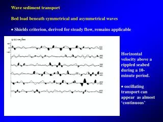
Wave sediment transport Bed load beneath symmetrical and asymmetrical waves Shields criterion, derived for steady flow, remains applicable Horizontal velocity above a rippled seabed during a 10-minute period. oscillating transport can appear as almost ‘continuous’

E N D
Wave sediment transport Bed load beneath symmetrical and asymmetrical waves Shields criterion, derived for steady flow, remains applicable Horizontal velocity above a rippled seabed during a 10-minute period. oscillating transport can appear as almost ‘continuous’
Instantaneous bed load transport empirical transport rate formulae for steady flow may be applied instant by instant through wave cycle time-averaging results gives net sand transport rate for symmetrical waves no net motion
Net bed load transport beneath steep [Stokes 2nd Order] waves Regions of validity for various wave theories: H = wave height, h = water depth T = wave period g = accel. due to gravity Stokes 2nd-order theory: most usually applied in ‘intermediate’ or ‘transitional’ water depth • correction 2to linear wave profile 1of magnitude proportional to wave steepness (ak)
The near-bed velocity amplitude (first harmonic) for a sinusoidal wave is given by: where a = H/2 = amplitude of surface elevation The corresponding peak Shields parameter during the wave cycle is: Using Soulsby’s (1997) friction factor: yields the peak Shields parameter (skin friction) for a sine wave as:
Beneath asymmetrical (Stokes 2nd Order) waves the velocity, and hence bed shear stress, are asymmetrical: The wave velocity may be expressed: where the asymmetry parameter W is given by:
We now make the assumption of quasi-steadiness with regard to the bed shear stress and assume that the instantaneous Shields parameter is given by: (Quadratic friction) • What is the net bed load sediment transport rate? • Here we make an unsteady application of Soulsby’s bed load formula derived for steady flow: For sheet flow conditions assume that θ>>θcr such that the Einstein parameter becomes: and hence Using this simplified formula the time-mean or net bed load transport, Qb, can be expressed as:
Class Exercise 6:By evaluating the integral , show that the net bed load transport rate is given by: This shows that the net bed load transport rate is proportional to the asymmetry parameter W. Recall that the result has neglected the threshold of sediment motion.
Suspended load beneath symmetrical and asymmetrical waves • entrainment occurs above both rippled and plane beds (i) Oscillating sheet flow measured with conductivity concentration meter (CCM) Large symmetrical waves: U0 = 1.7 ms-1 T = 7.2 s D50 = 0.21 mm Delft Hydraulics Ribberink and Al Salem (1992)
Intra-wave concentrations measured (with OPCON probe) at three heights in suspension layer Cycle-mean concentration profiles (power law profiles: straight lines on log-log plot)
Cycle-mean concentration profile • above plane beds simplified form of the Rouse profile: • vertical profile of cycle-mean concentration <C> has slope m = 1/2 on log-log plot • m has the form of Rouse parameter • Suspension above rippled beds • entrainment is dominated by vortex formation and shedding in a near-bed layer of thickness equivalent to about 2 ripple heights • effective convective mechanism for transporting sediment to significantly greater heights than above plane beds • vortex shedding becomes important if the ripple steepness
Vortex shedding beneath symmetrical waves net transport above ripples depends upon degree of asymmetry in the wave motion Vortex shedding beneath asymmetrical waves vortex shedding gives rise to net transport in direction opposite to that of wave advance (c.f. flat bed case)
Cycle-mean concentration profile above rippled beds despite convective nature of the vortex shedding process, mean C-profile is usually modelled using diffusive concepts: [Upward diffusion + Settling = 0] < ..> = ‘cycle-mean’ s = sediment diffusivity s = constant due to uniformity of vertical mixing in near-bed layer above ripples in which decay scale Lr is related to ripple height
Bed forms in oscillatory flow Parameters involved in ripple formation at low flow stages Ripples in sinusoidal oscillatory flow are generally long-crested symmetrical regularly spaced with crests transverse to plane of the orbital motion Ripple development: development of initially flat bed as orbital diameter d0increases threshold of motion exceeded θ' ≥ 0.045 first stage of ripple formation initiated for small d0, ripple wavelength d0 e.g
ripple steepness gradually increases until “vortex” ripples develop with steepness 0.15≤ /λ≤ 0.2 • flow separates in each wave cycle • ripples attain a maximum steepness, (/λ )max = 0.2 - 0.22, and crest angles (up to 120) Field observations of ripple wavelength
at very high flow stages (θSF≥ 1), ripples are “washed out” and bed flattens • substantial suspended load confined to thin oscillating “sheet flow” layer • seabed is ‘self regulating’ i.e. transport rates are ‘capped’ beneath large (e.g. storm) waves • Empirical formulae for ripple prediction : e.g. Nielsen (1992). • Field observations • wave-generated ripples are widespread on the continental shelf • (depths up to 50-100m) • natural surface waves are irregular ripple properties are determined by wave spectrum • ripple formation may be occasional (i.e. as a result of higher waves) ‘fossil’ or ‘relict’ ripples often remain in low wave conditions
Field observations (cont.) Occurrence of ripples in the field Threshold of motion is denoted by M = Mc M = Mobility number maximum ripple wavelengths < those in the laboratory (for same sand size) ripples formed by irregular waves are less steep than those formed by regular waves bed roughness is less than expected from laboratory
Morphological modelling (for ripples) • prediction of evolution of bed as a result of divergence in predicted sediment transport rate, e.g. Shear stress and transport distribution over surface of a ripple in steady flow • maximum bed shear stress (skin friction) occurs just upstream of crest critical condition for ripple growth • ripple profile will grow or be eroded locally according to sediment continuity equation : n = porosity of bed • if , then i.e. the bed level rises, and vice versa • advection-diffusion of sediment in suspension should also be included in a comprehensive scheme
Wave-current interaction in the seabed boundary layer • combined effects of waves and currents represents general situation on continental shelf • waves modify the tidal dynamics (i.e. alter mean currents) only in shallow coastal waters (depth h<30m), but potentially affect sediment transport rates over entire shelf • continuum of conditions arises between earlier limiting cases of (i) Currents Alone and (ii) Waves Alone: • STEADY Small Waves Large Waves WAVES • CURRENT on a on a • ALONE Strong Current Weak Current ALONE e.g. composite drag coefficients / friction factors necessary for practical purposes: CD Combined fw CURRENTS Friction/Drag WAVES ALONE Coefficient ALONE
in bottom seabed boundary layer, waves and currents interact nonlinearly, • e.g. turbulent kinetic energy (T.K.E.) : • e.g. cycle-mean bed shear stress: • i.e. waves enhance the current-generated stresses Cycle-mean velocity profile in W + C flow
Prediction of sediment • transport rates by W + C • peak bed shear stress in the wave cycle is often of central importance: • earlier considerations for currents alone and waves alone remain applicable, with modifications for wave-current interaction • roughly speaking, waves stir up the bottom sediment while current transports the sediment
Practical sand transport model TRANSPOR Van Rijn (1993) This is a process-based (algebraic not numerical) approach. Predicted transport rates in perpendicularly combined W + C flow TRANSPOR has been parameterised to produce the simpler Soulsby-Van Rijn formula (Soulsby, 1997)
Soulsby-Van Rijn formula (see Soulsby, 1997) where with and = depth-averaged current = root-mean-square wave orbital velocity = drag coefficient due to current alone = threshold current velocity given by Van Rijn (1984): for for
SI units must be used in the above equations = slope of bed in streamwise direction, positive if flow runs uphill h = water depth d50 = median grain diameter z0 = bed roughness length = 0.006 m s = relative density of sediment g = acceleration due to gravity = kinematic viscosity of water D* = non-dimensional grain diameter The formula applies to total (bed plus suspended load) transport in combined W+C on horizontal and sloping beds. Term Asb gives the bed load, and term Ass the suspended load transport. The method is intended for conditions in which the bed is rippled, and z0 should be set to 6mm. It was derived by applying the principles of Grass (1981) who developed one of the first W+C formulations, and it was calibrated against the transport curves plotted by van Rijn (see previous sheet) based on the TRANSPOR program. TRANSPOR itself was calibrated using various field data. The bed slope term (1-1.6tan) is a commonly used device, but is a less correct procedure than modifying the threshold velocity for slope effects.
What governs long-term sediment transport patterns on the continental shelf? effect of waves on transport rates on site varies from day to day, and seasonally largest contributions to long-term transport are due to fairly large, frequently occurring waves combined with currents lying between mean spring- and neap-maxima extreme events (e.g. major storms occurring during spring tides) do not dominate long-term transport, as often supposed