Download
1 / 66
670 likes | 1.96k Vues
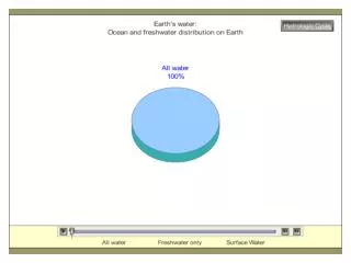
mP. cP. mT. cT. Review questions:. Describe the movement of water through the hydrologic cycle. . Most water evaporates from the oceans. Some of the water is transported considerable distances, condenses to form clouds, and eventually falls to earth’s surface as precipitation.

E N D
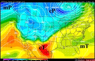
mP cP mT cT
Review questions: Describe the movement of water through the hydrologic cycle. • Most water evaporates from the oceans. • Some of the water is transported considerable distances, condenses • to form clouds, and eventually falls to earth’s surface as • precipitation. • Once precipitation has fallen on land, some reenters the atmosphere • by evaporation and transpiration, some soaks in and some runs off. • The water that soaks in or runs off eventually makes is way back • to the ocean to begin the cycle again.
Review questions: How does stable air differ from unstable air? • Stable air resists vertical motion whereas unstable air • reinforces vertical motion.
Review questions: Why are high clouds always thin in comparison to low or middle clouds? • High clouds are always thin because of the low • temperatures and thus the small quantity of water vapor • available at the altitudes where they form
Review questions: Explain why air pressure decreases with an increase in altitude. • Air pressure is exerted by the weight of air above. • Air pressure decreases with an increase in altitude because, as one moves away from the Earth’s surface, there is less air above to exert a downward force.
Chapter 12 Weather Analysis and Forecasting -The Weather Business -Weather Analysis -Weather Forecasting -Long Range Forecasts -Forecasting Accuracy -Tools in Weather Forecasting
Now Then
The Weather Business In the United States, the governmental agency responsible for gathering and disseminating weather related information is the National Weather Service (NWS). The most important services provided by the NWS are forecasts and warnings of hazardous weather information including: thunderstorms, flooding, hurricanes, tornadoes, winter weather and extreme heat. Weather forecasting is the process, (science, art) by which, from current weather patterns, various methods are used to determine the state of the atmosphere.
The National Weather Service is responsible for issuing forecasts and warnings of hazardous weather including thunderstorms, flooding, hurricanes…..
One of the responsibilities of the NWS is river flood forecasting
Just like weather forecasting, constant data collection is routine
Large Rivers are monitored at several key locations to assess changes in river flow.
Stream Gaging By using automated equipment in the gaging station, river stage can be continuously monitored and reported to an accuracy of 1/8 of an inch. Linking battery-powered stage recorders with satellite radios enables transmission of stage data to computers in USGS and NWS facilities even when extreme high waters and strong winds disrupt normal telephone and power services. In this way, USGS and NWS hydrologists know the river stage at remote sites and how fast the water is rising or falling.
Typical NWS product To produce the image shown above is very complicated, labor intensive undertaking.
The Weather Business To produce even a short range forecast involves numerous steps, including collecting weather data, compiling it on a global scale, and transmitting it. The NWS is not responsible for the plethora of animated weather images we see on TV. It is not part of the mission of the NWS to provide these data. Private enterprises, using “raw data” from the NWS, undertake this task. It is a unique joint venture between the NWS and the private weather sector. The NWS is the official voice, and therefore is ultimately responsible in the United States for issuing warnings.
Weather Analysis Before issuing a forecasting, the forecaster must have an accurate picture of the atmospheric conditions; this project is called the weather analysis. Because the atmosphere is always changing, time is of the essence when analyzing the weather. Clearly, high speed computers have revolutionized the weather analysis process. First introduced in 1985, this system had a peak performance of 1.9 gigaflops. At the time, the CRAY-2 system had the world's largest central memory with the possibility of 2048 megaBytes, which is still considered large today.
Gathering Data A critical mass of information is needed to generate a useful weather chart for even a short range forecast. The World Meteorological Organizationwhich includes more than 130 nations, was formed to address this problem. It is their responsibility for gathering the needed data and for producing numerous weather maps and upper-level charts that describe the current state of the atmosphere.
Information is collected by the WMO then transmitted to three World Meteorological Centers. From there the world centers send data to the meteorological center in each office. Washington, DC Geneva, Switzerland Moscow, Russia Melbourne, Australia
Weather Maps: Pictures of the Atmosphere Once weather data has been collected, the analyst displays it on a number of different synoptic weather maps which are used to produce weather forecasts. Synoptic means coincident in time. (syn- same, optic – to look at) (Of or relating to data obtained nearly simultaneously over a large area of the atmosphere) Over 200 surface maps and charts are produced by the NWS and its forecast centers. As we already know, different levels in the atmosphere are used to study different processes important to weather forecasting….
Surface Maps Surface maps show the location of major pressure centers, fronts, weather conditions at several locations.
850-millibar Maps CAA WAA 850-mb maps are useful to analyze temperature advection and observe surface features.
700-millibar Maps 700-mb maps are useful to track the movement of air-mass thunderstorms.
500-millibar Maps L L L H 500-mb maps are useful to predict the movement of upper level cyclones. Prior to high-speed computing 500-millibar maps were heavily relied on.
300-millibar Maps 300 (200mb) maps show jet stream location. Recall the jet stream associated with areas of upper level divergence and convergence.
The Challenge of Forecasting (pg 324) Imagine a system on a rotating sphere that is 8000 miles wide, consisting of different materials, different gases that have different properties (one of the most important of which is water which is exists in different concentrations), heated by a nuclear reactor 93 million miles away.Then just to make life interesting, this sphere is oriented such that as it revolves around the reactor it is heated differently at different locations at different times of the year: Then someone is asked to watch the mixture of gases, a fluid only 20 miles deep, that covers an area of 250 million square miles, and to predict the state of that fluid at one point on a sphere 2 days from now. This is the problem forecaster have to face. (Bob Ryan WRC-TV)
Synoptic Weather Forecasting • Until the late 1950’s synoptic weather forecasting was the • primary basis for weather prediction. Forecasters relied • heavily on synoptic weather maps to forecast. • Other methods of weather forecasting include: • Persistence Forecasting: yesterday’s weather today • Trend Forecasting: similar to persistence with slight changes in previous day’s weather • Analog Approach: current weather conditions are matched with records of similar past weather events (Model Output Statistics).
The persistence method assumes that the conditions at the time of the forecast will not change. For example, if it is sunny and 87 degrees today, the persistence method predicts that it will be sunny and 87 degrees tomorrow. If two inches of rain fell today, the persistence method would predict two inches of rain for tomorrow.
The trends method involves determining the speed and direction of movement for fronts, high and low pressure centers, and areas of clouds and precipitation.
Numerical Weather Prediction Numerical weather prediction relies on the fact that the gases of the atmosphere obey a number of known physical principles. (PV=nRT for example) Numerical weather prediction employs a number of highly refined computer models to attempt to mimic the behavior of the atmosphere. Using numerical models, the National Weather Service produces a number of prognostic charts whichpredict the state of the atmosphere in the future (temperature, winds, moisture, clouds, precipitation).
History of Numerical Weather Prediction • 1775 equations of fluid mechanics were formulated • (Leonhard Euler) • 1827 terms for molecular viscosity were added • (Cluade-Louis Navier), (George Stokes) in 1845. The • Navier-Stokes equations. • 1888 rough equations developed by Stokes and • Navier were refined by Helmhotz. • 1922 Lewis Fry Richardson published a book describing the • first experimental NWP. (took 6weeks for a 6 hr forecast) • Surface pressure was way off. Not deemed feasible; no • work done for almost 2 decades.
History of Numerical Weather Prediction • 1945 Physicists (John von Neuman) at Princeton and RCA’s Princeton Laboratories (Zworykin) proposed to initiate NWP using the electronic computers. Simulate general circulation. Very hard time agreeing how to approach the problem. • Major Players (Carl-Gustav Rossby, Arnt Eliassen, Jule Charney, and George Platzman)…decided they needed to simplify the full primitive equations to focus on the long waves of general circulation.
Electronic Numerical Integrator And Computer The ENIAC machine occupied a room thirty by fifty feet. The controls are at the left, and a small part of the output device is seen at the right.
History of Numerical Weather Prediction • 1948-1949 Charney and von Neuman presented results from a simple barotropic model at NWP conferences. • (machine code, domain size?, many calculations done with slide rule and mechanical calculators) • 1950 Electronic Numerical Integrator and Computer ENIAC forecasts were made (three case studies). Results were promising. Swedish computer “BESK” became operational in 1953 • 1954 With Swedish Air Force support 24, 48 and • later 72hr forecasts of 50 kPa Heights (not surface • conditions)
History of Numerical Weather Prediction • 1953 IBM announced specifications for a new computer. • 1954 US Weather Bureau, USAF Weather Service formed • the Joint Numerical Weather Prediction Unit (JNWPU). • Operational weather forecasts using a quasi-geostrophic • baroclinic model developed by Charney and Eliassen). • Three layer 40, 70, and 90 kPa. • 1955 IBM 701 was introduced; Panofsky proposed a • scheme for automated analysis of weather data.
History of Numerical Weather Prediction • 1955-57 Loss of personnel limited the growth of the • JNWPU. Weather forecasts were of poor quality and not • appreciated by experienced forecasters. During the • first two years the forecasts were largely ignored. • 1958 National Meteorological Center (NMC) • formed to run NWS operational weather models. • 1958 USAF GWC (Omaha, NE) NAVY FNWC • (Monterey, CA) formed.
History of Numerical Weather Prediction • At first numerical forecasts were initializied with hand-analyzed data • Mid 1950’s an objective analysis method was adopted (fitting new observations to previous forecast fields) • 1955,1956 first attempt at a baroclinic (multi-layer) model failed because it was poorly calibrated and awkward to use • Revert back to one layer barotropic domain…computer power now underutilized!! • To better use power of the computer the domain of the barotropic model was expanded
History of Numerical Weather Prediction • The models (because they lacked sufficient topography) did not produce realistic results in the westward movement of longwaves in the general circulation pattern. Removal and reinsertion (after fudging) of the longest waves was the work around…..challenging times in NWP • 1963 faster computers lead to six layer primitive equation models. Forecast scores improved dramatically. • Since the mid 60’s improvements in forecast quality has been closely tied to computer power. • -more grid points, more vertical layers, larger domain • -topography, landscape, snow/ice coverage • -radiation, precipitation, clouds, turbulence
Current Numerical Weather Prediction Models • There are four computer models that are run by the National Centers for Environmental Prediction (NCEP) which are used for forecasting the day-to-day weather in the United States: • Nested Grid model (NGM) 1990 • Eta Model early 1990’s • Global Forecast System (GFS) • Rapid Update Cycle (RUC) • Each model is a self-contained set of computer programs which include means of analyzing data and computing the evolution of the atmosphere's winds, temperature, pressure, and moisture based on the analyses. • These individual models are all quite different from each other in one essential aspect or another, either in their formulation or their implementation.
Current NCEP Numerical Weather Prediction Models • GFS (formerly the MRF) • Became operational in 1985. • It is a Global Spectral Model. • A spectrum of waves in the atmosphere is represented by • sine and cosine functions rather than specific grid point • values. • - Momentum Equation • - Thermodynamic Equation • - Continuity Equation • - Moisture Equation (transport, sources, sinks) • - Hydrostatic Equation
Eta Model The number and distribution of vertical layers in the operational Eta Model has changed throughout the years Implemented in 1993 (0-48hrs) 80km resolution Oct 1995 Eta -48km w/EDAS Feb 1998 Eta –32km (0000, 1200 UT) 48 hr forecast 3D var Mar 1995 Eta –29km (meso Eta) (0300 and 1500 UT) Feb 1998 Eta –32km (0300 + 1800UT) 45 levels 2001 Eta –12km 60 layers
Eta Model Vertical Resolution Characteristics/Layer Distribution
Vertical Coordinates A model’s vertical structure is as important in defining the model’s behavior as the horizontal configuration and model type. Proper depiction of the vertical structure requires selection of an appropriate vertical coordinate and sufficient vertical resolution. Two Common Vertical Coordinates: Sigma Vertical Coordinate (NGM, AVN/GFS, ECMWF, NOGAPS and UKMET, MM5, COAMPS, RAMS) Eta (or Step) Vertical Coordinate
In its simplest form , the sigma coordinate is defined by = p/ps p is the pressure on a forecast level within the model and ps is the pressure at the earth’s surface, not mean sea level pressure. The lowest coordinate surface ( = 1) follows a smoothed version of the actual terrain.
Sigma Vertical Coordinate ( ) To address the problem of discontinuous forecast surfaces, Phillips (1957) developed a terrain-following coordinate called the sigma ( ) coordinate, illustrated below. The sigma coordinate or variants are used in the NGM, AVN/MRF, ECMWF, NOGAPS, and UKMET models and appear in some meso-scale models, such as AFWA MM5, COAMPS, and RAMS.
Advantages of the Sigma Vertical Coordinate • Advantages: • Since the sigma coordinate is related to pressure, it produces relatively simple formulations for handling the lower boundary without overly complicating the equations of motion. The simplified formulations are easier to program. • The terrain-following nature of the sigma coordinate lends itself to increasing vertical resolution near the ground consistently over the full model domain. The model can better define boundary-layer processes and features that contribute to sensible weather elements (diurnal heating, low-level winds/turbulence/moisture)
1) Model wind forecasts depend on accurate calculation of the pressure gradient force (PGF). When sigma surfaces slope, the PGF must be expanded from its simple pressure coordiante form account for the slope. This can introduce errors because the lapse rate must be expanded approximated at points that lie between the pressure surfaces. With steep slopes the errors can be significant. 2) Because the actual and often abrupt steepness of mountain slopes is smoothed in sigma coordinate models, they often misrepresent the true surface elevation. This can cause forecasts for locations immediately adjacent to mountain ranges to severely misrepresent the surface pressure and thus the temperature and moisture (PGF as well). Limitations of the Sigma Vertical Coordinate