Download
1 / 27
270 likes | 290 Vues
Learn how to calculate the slope and y-intercept in linear regression, and understand the logic and assumptions behind One-Way ANOVA for comparing means in different groups.

E N D
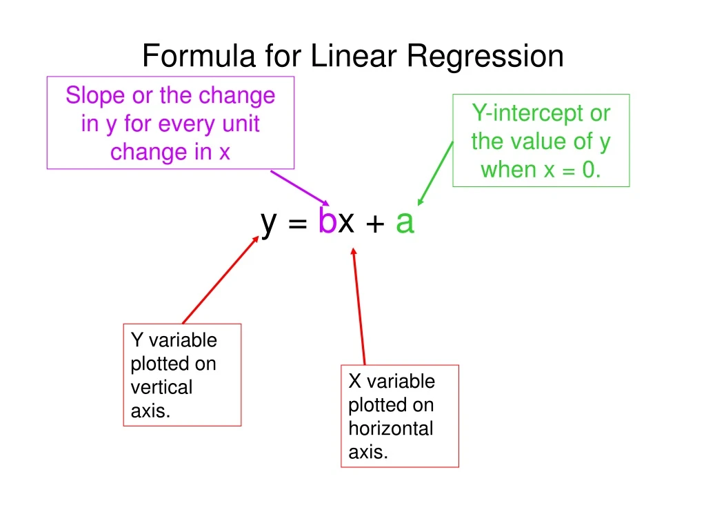
Formula for Linear Regression Slope or the change in y for every unit change in x Y-intercept or the value of y when x = 0. y = bx + a Y variable plotted on vertical axis. X variable plotted on horizontal axis.
Interpretation of parameters • The regression slope is the average change in Y when X increases by 1 unit • The intercept is the predicted value for Y when X = 0 • If the slope = 0, then X does not help in predicting Y (linearly)
General ANOVA SettingComparisons of 2 or more means • Investigator controls one or more independent variables • Called factors (or treatment variables) • Each factor contains two or more levels (or groups or categories/classifications) • Observe effects on the dependent variable • Response to levels of independent variable • Experimental design: the plan used to collect the data
Logic of ANOVA • Each observation Mean is different from the Grand (total sample) Mean by some amount • There are two sources of variance from the mean: • 1) That due to the treatment or independent variable • 2) That which is unexplained by our treatment
One-Way Analysis of Variance • Evaluate the difference among the means of two or more groups Examples: Accident rates for 1st, 2nd, and 3rd shift Expected mileage for five brands of tires • Assumptions • Populations are normally distributed • Populations have equal variances • Samples are randomly and independently drawn
Hypotheses of One-Way ANOVA • All population means are equal • i.e., no treatment effect (no variation in means among groups) • At least one population mean is different • i.e., there is a treatment effect • Does not mean that all population means are different (some pairs may be the same) • ANOVA does not tell you where the difference lies. For this reason ,you need another test, either the Scheffe' or Tukey post ANOVA test.
One-Factor ANOVA All Means are the same: The Null Hypothesis is True (No Treatment Effect)
One-Factor ANOVA (continued) At least one mean is different: The Null Hypothesis is NOT true (Treatment Effect is present) or
Partitioning the Variation • Total variation can be split into two parts: SST = SSA + SSW SST = Total Sum of Squares (Total variation) SSA = Sum of Squares Among Groups (Among-group variation) SSW = Sum of Squares Within Groups (Within-group variation)
Partitioning the Variation (continued) SST = SSA + SSW Total Variation = the aggregate dispersion of the individual data values across the various factor levels (SST) Among-Group Variation = dispersion between the factor sample means (SSA) Within-Group Variation = dispersion that exists among the data values within a particular factor level (SSW)
Commonly referred to as: Sum of Squares Within Sum of Squares Error Sum of Squares Unexplained Within-Group Variation Partition of Total Variation Total Variation (SST) d.f. = n – 1 Variation Due to Factor (SSA) Variation Due to Random Sampling (SSW) + = d.f. = c – 1 d.f. = n – c Commonly referred to as: • Sum of Squares Between • Sum of Squares Among • Sum of Squares Explained • Among Groups Variation
Among-Group Variation (continued) Variation Due to Differences Among Groups Mean Square Among = SSA/degrees of freedom
Within-Group Variation (continued) Summing the variation within each group and then adding over all groups Mean Square Within = SSW/degrees of freedom
One-Way ANOVA Table Source of Variation MS (Variance) SS df F ratio SSA Among Groups MSA SSA c - 1 MSA = F = c - 1 MSW SSW Within Groups SSW n - c MSW = n - c SST = SSA+SSW Total n - 1 c = number of groups n = sum of the sample sizes from all groups df = degrees of freedom
One-Way ANOVA: F Test Statistic • Test statistic MSA is mean squares among groups MSW is mean squares within groups • Degrees of freedom • df1 = c – 1 (c = number of groups) • df2 = n – c (n = sum of sample sizes from all populations) H0: μ1= μ2 = …= μc H1: At least two population means are different
Interpreting One-Way ANOVAF Statistic • The F statistic is the ratio of the among estimate of variance and the within estimate of variance • The ratio must always be positive • df1 = c -1 will typically be small • df2 = n - c will typically be large Decision Rule: • Reject H0 if F > FU, otherwise do not reject H0 = .05 0 Do not reject H0 Reject H0 FU
You want to see if cholesterol level is different in three groups. You randomly select five patients. Measure their cholesterol levels. At the 0.05 significance level, is there a difference in mean cholesterol? One-Way ANOVA : F Test Example Gp 1Gp 2Gp 3 254 234 200 263 218 222 241 235 197 237 227 206 251 216 204
One-Way ANOVA Example: Scatter Diagram Cholesterol 270 260 250 240 230 220 210 200 190 Gp 1Gp 2Gp 3 254 234 200 263 218 222 241 235 197 237 227 206 251 216 204 • • • • • • • • • • • • • • • 1 2 3 Groups
One-Way ANOVA Example Computations Gp 1Gp 2Gp 3 254 234 200 263 218 222 241 235 197 237 227 206 251 216 204 X1 = 249.2 X2 = 226.0 X3 = 205.8 X = 227.0 n1 = 5 n2 = 5 n3 = 5 n = 15 c = 3 SSA = 5 (249.2 – 227)2 + 5 (226 – 227)2 + 5 (205.8 – 227)2 = 4716.4 SSW = (254 – 249.2)2 + (263 – 249.2)2 +…+ (204 – 205.8)2 = 1119.6 MSA = 4716.4 / (3-1) = 2358.2 MSW = 1119.6 / (15-3) = 93.3
H0: μ1 = μ2 = μ3 H1: μj not all equal = 0.05 df1= 2 df2 = 12 One-Way ANOVA Example Solution Test Statistic: Decision: Conclusion: Critical Value: FU = 3.89 Reject H0 at = 0.05 = .05 There is evidence that at least one μj differs from the rest 0 Do not reject H0 Reject H0 F= 25.275 FU = 3.89
Significant and Non-significant Differences Non-significant: Within > Between Significant: Between > Within
ANOVA (summary) • Null hypothesis is that there is no difference between the means. • Alternate hypothesis is that at least two means differ. • Use the F statistic as your test statistic. It tests the between-sample variance (difference between the means) against the within-sample variance (variability within the sample). The larger this is the more likely the means are different. • Degrees of freedom for numerator is k-1 (k is the number of treatments) • Degrees of freedom for the denominator is n-k (n is the number of responses) • If test F is larger than critical F, then reject the null. • If p-value is less than alpha, then reject the null.
ANOVA (summary) WHEN YOU REJECT THE NULL For an one-way ANOVA after you have rejected the null, you may want to determine which treatment yielded the best results. Must do follow-on analysis to determine if the difference between each pair of means if significant (post ANOVA test).
One-way ANOVA (example) The study described here is about measuring cortisol levels in 3 groups of subjects : • Healthy (n = 16) • Depressed: Non-melancholic depressed (n = 22) • Depressed: Melancholic depressed (n = 18)
Results • Results were obtained as follows Source DF SS MS F P Grp. 2 164.7 82.3 6.61 0.003 Error 53 660.0 12.5 Total 55 824.7 Individual 95% CIs For Mean Based on Pooled StDev Level N Mean StDev -+---------+---------+---------+----- 1 16 9.200 2.931 (------*------) 2 22 10.700 2.758 (-----*-----) 3 18 13.500 4.674 (------*------) -+---------+---------+---------+----- Pooled StDev = 3.529 7.5 10.0 12.5 15.0
Multiple Comparison of the Means - 1 • Several methods are available depending upon whether one wishes to compare means with a control mean(Dunnett) or just overall comparison (Tukey and Fisher) Dunnett's comparisons with a control Critical value = 2.27 Control = level (1) of Grp. Intervals for treatment mean minus control mean Level Lower Center Upper -----+---------+---------+---------+-- • 2 -1.127 1.500 4.127 (----------*----------) • 3 1.553 4.300 7.047 (----------*----------) • -----+---------+---------+---------+-- -1.0 1.5 4.0 7.0
Multiple Comparison of Means - 2 Tukey's pair wise comparisons Intervals for (column level mean) − (row level mean) • 1 2 • 2 -4.296 • 1.296 • 3 -7.224 -5.504 • -1.376 -0.096 Fisher's pair wise comparisons Intervals for (column level mean) − (row level mean) • 1 2 • 2 -3.826 • 0.826 • 3 -6.732 -5.050 • -1.868 -0.550 The End