Download
1 / 19
190 likes | 221 Vues
This comprehensive text delves into the material description of fluid motion, evolution of moving fluid parcels and particles, and the importance of conservation laws in fluid mechanics. It explores the development of mathematical tools required for treating open systems, kinematic relations, and Reynolds transport theorem. The text covers the deformation of differential volumes over time, field quantities, material derivatives, and control volumes. It also introduces the material derivative of the Jacobian function and simplifies it based on transformation function derivatives. With self-study recommendations, this resource is invaluable for understanding the kinematics of fluid motion.

E N D
Development of Conservation Equations for A CV P M V Subbarao Professor Mechanical Engineering Department I I T Delhi Comprehensive Description of Fluid Flows……
Material description of a fluid particle motion. The motion of a fluid particle with respect to a reference coordinate system is in general given by a time dependent position vector x(t)
Evolution of Shape of Moving Particle Material derivative of Jcabian:
Comprehensive Description • The conservation laws in integral form are, strictly speaking, valid for closed systems. • Fluid mechanics deals with open systems, where the mass flow continuously crosses the system boundary. • To apply the conservation laws to open systems, sepecial necessary mathematical tools need to be developed. • These tools help in treating the volume integral of an arbitrary field quantity f(x,t). • An important kinematic relation to develop a generalized mathematical models for fluid flows.
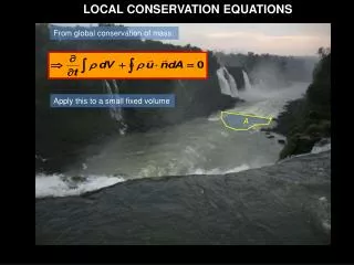
The control mass occupies region I and C.V. (region II) at time t0. Fluid particles of region – I are trying to enter C.V. (II) at time t0. Reynolds Descriptions a System • the same control mass occupies regions (II+III) at t0 + dt • Fluid particles of I will enter CV-II in a time dt. • Few more fluid particles which belong to CV – II at t0 will occupy III at time t0 + dt.
III II At time t0+dt II I At time t0 Reynolds' Transport Theorem I has entered and III has left CV at time t0+dt I is trying to enter CV at time t0 The control volume may move as time passes.
Deformation of a differential volume at differentinstant of time
The Field quantity • The field quantity f(x,t) may be a zeroth, first or second order tensor valued function. • Namely, as mass, concentration, velocity vector, and stress tensor. • A fluid element of given initial volume (dV0) may change its volume and/or change it surface (ds0) with a given time, while moving through the flow field. • This is due to various experiences by the element namely, dilatation, compression and deformation. • Let us consider the same fluid particles at any time and therefore, it is called the material volume.
Change in Field quantity of A Control Volume The total value of a field quantity for a CV. volume integral of the quantity f(x,t): This is a function of time only. The integration must be carried out over the varying volume V(t). The material change of the quantity F(t) is expressed as: Since the shape of the volume V(t) changes with time, the differentiation andintegration cannot be interchanged.
Reynolds analogy permits the transformation of the time dependent volume V(t) into the fixed volume V0 at time t = 0 by using the Jacobian transformation function: The Fundamental Reynolds Analogy
Change in Field quantity of A Control Volume With this operation it is possible to interchange the sequence of differentiation and integration: The chain differentiation of the expression within the parenthesis results in
Material Derivative of Jocobian Function • Every volume element dV follows the motion from x=f(, t) to x=f(, t+dt) and changes its shape and size. • As a result, the Jacobian transformation function undergoes a time change. • This change is the material derivative of J: Self Study : Chapter 3 : Kinematics of Fluid Motion Fluid Mechanics for Engineers
Introducing the material derivative of the Jacobian function and simplifying based on derivatives of transformation functions This equation permits the back transformation of the fixed volume integral into the time dependent volume integral.
The chain rule applied to the second and third term yields: The second volume integral in above equation can be converted into a surface integral by applying the Gauss' divergence theorem:
This Equation is valid for any system boundary with time the dependent volume V(t) and surface s(t) at any time. Also valid at the time t = t0 , where the volume V = VCand the surface s = sC. VC and sC are named as control volume and control surface. These control surfaces can be inlets or exits.