Download
1 / 59
590 likes | 621 Vues
Explore the mysterious dark energy through cosmic observations and the subtle but crucial acoustic oscillations in the universe. Learn about the challenges in measuring and comparing cosmologies. Delve into the statistical signals and the profound implications of acoustic peaks in understanding the cosmos.

E N D
Dark Energy and Cosmic Sound Daniel Eisenstein (University of Arizona) Michael Blanton, David Hogg, Bob Nichol, Nikhil Padmanabhan, Will Percival, David Schlegel, Roman Scoccimarro, Ryan Scranton, Hee-Jong Seo, Ed Sirko, David Spergel, Max Tegmark, Martin White, Idit Zehavi, and the SDSS.
Dark Energy is Mysterious • Observations suggest that the expansion of the universe is presently accelerating. • Normal matter doesn’t do this! • Requires exotic new physics. • Cosmological constant? • Very low mass field? • Some alteration to gravity? • We have no compelling theory for this! • Need observational measure of the time evolution of the effect.
dr = (c/H)dz dr = DAdq Observer A Quick Distance Primer • The homogeneous metric is described by two quantities: • The size as a function of time,a(t). Equivalent to the Hubble parameter H(z) = d ln(a)/dt. • The spatial curvature, parameterized by Wk. • The distance is then (flat) • H(z) depends on the dark energy density.
Dark Energy is Subtle • Parameterize by equation of state, w = p/r, which controls how the energy density evolves with time. • Measuring w(z) requires exquisite precision. • Varying w assuming perfect CMB: • Fixed Wmh2 • DA(z=1000) • w(z) is even harder. • Need 1% distance measurements! Comparing Cosmologies
Outline • Baryon acoustic oscillations as a standard ruler. • Detection of the acoustic signature in the SDSS Luminous Red Galaxy sample at z=0.35. • Cosmological constraints therefrom. • Large galaxy surveys at higher redshifts. • Future surveys could measure H(z) and DA(z) to better than 1% from z=0.3 to z=3. • Present the Baryon Oscillation Spectroscopic Survey and SDSS-III. • Assess the leverage on dark energy and compare to alternatives.
Acoustic Oscillations in the CMB • Although there are fluctuations on all scales, there is a characteristic angular scale.
Acoustic Oscillations in the CMB WMAP team (Bennett et al. 2003)
Before recombination: Universe is ionized. Photons provide enormous pressure and restoring force. Perturbations oscillate as acoustic waves. After recombination: Universe is neutral. Photons can travel freely past the baryons. Phase of oscillation at trec affects late-time amplitude. Recombination z ~ 1000 ~400,000 years Big Bang Neutral Ionized Today Time Sound Waves in the Early Universe
Sound Waves • Each initial overdensity (in DM & gas) is an overpressure that launches a spherical sound wave. • This wave travels outwards at 57% of the speed of light. • Pressure-providing photons decouple at recombination. CMB travels to us from these spheres. • Sound speed plummets. Wave stalls at a radius of 150 Mpc. • Overdensity in shell (gas) and in the original center (DM) both seed the formation of galaxies. Preferred separation of 150 Mpc.
A Statistical Signal • The Universe is a super-position of these shells. • The shell is weaker than displayed. • Hence, you do not expect to see bullseyes in the galaxy distribution. • Instead, we get a 1% bump in the correlation function.
Remember: This is a tiny ripple on a big background. Response of a point perturbation Based on CMBfast outputs (Seljak & Zaldarriaga). Green’s function view from Bashinsky & Bertschinger 2001.
Acoustic Oscillations in Fourier Space • A crest launches a planar sound wave, which at recombination may or may not be in phase with the next crest. • Get a sequence of constructive and destructive interferences as a function of wavenumber. • Peaks are weak — suppressed by the baryon fraction. • Higher harmonics suffer from Silk damping. Linear regime matter power spectrum
Acoustic Oscillations, Reprise • Divide by zero-baryon reference model. • Acoustic peaks are 10% modulations. • Requires large surveys to detect! Linear regime matter power spectrum
dr = (c/H)dz dr = DAdq Observer A Standard Ruler • The acoustic oscillation scale depends on the sound speed and the propagation time. • These depend on the matter-to-radiation ratio (Wmh2) and the baryon-to-photon ratio (Wbh2). • The CMB anisotropies measure these and fix the oscillation scale. • In a redshift survey, we can measure this along and across the line of sight. • Yields H(z) and DA(z)!
Galaxy Redshift Surveys • Redshift surveys are a popular way to measure the 3-dimensional clustering of matter. • But there are complications from: • Non-linear structure formation • Bias (light ≠ mass) • Redshift distortions • Do these affectthe acousticsignatures? SDSS
Nonlinearities & Bias • Non-linear gravitational collapse partially smears out the signature (more later). • Clustering bias and redshift distortions alter the power spectrum but don’t create preferred scales at 150 Mpc! • Acoustic peaks expected to survive mostly intact. z=1 Meiksen & White (1997), Seo & DJE (2005)
Virtues of the Acoustic Peaks • The acoustic signature is created by physics at z=1000 when the perturbations are 1 in 104. Linear perturbation theory is excellent. • Measuring the acoustic peaks across redshift gives a geometrical measurement of cosmological distance. • The acoustic peaks are a manifestation of a preferred scale. Still a very large scale today, so non-linear effects are mild and dominated by gravitational flows that we can simulate accurately. • No known way to create a sharp scale at 150 Mpc with low-redshift astrophysics. • Measures absolute distance, including that to z=1000. • Method has intrinsic cross-check between H(z) & DA(z), since DA is an integral of H.
Introduction to SDSS LRGs • SDSS uses color to target luminous, early-type galaxies at 0.2<z<0.5. • Fainter than MAIN (r<19.5) • About 15/sq deg • Excellent redshift success rate • The sample is close to mass-limited at z<0.38. Number density ~ 10-4h3 Mpc-3. • Science Goals: • Clustering on largest scales • Galaxy clusters to z~0.5 • Evolution of massive galaxies
Redshift Distribution 55,000 galaxies for this analysis; about 100k now available.
Intermediate-scale Correlations Redshift-space Real-space • Subtle luminosity dependence in amplitude. • s8 = 1.80±0.03 up to 2.06±0.06 across samples • r0 = 9.8h-1 up to 11.2h-1 Mpc • Real-space correlation function is not a power-law. Zehavi et al. (2004)
Acoustic series in P(k) becomes a single peak in x(r)! Pure CDM model has no peak. Warning: Correlated Error Bars Large-scale Correlations
Another View CDM with baryons is a good fit: c2= 16.1 with 17 dof.Pure CDM rejected at Dc2= 11.7
A Prediction Confirmed! • Standard inflationary CDM model requires acoustic peaks. • Important confirmation of basic prediction of the model. • This demonstrates that structure grows from z=1000 to z=0 by linear theory. • Survival of narrow feature means no mode coupling.
Equality scale depends on (Wmh2)-1. Wmh2 = 0.12 Wmh2 = 0.13 Wmh2 = 0.14 Acoustic scale depends on (Wmh2)-0.25. Two Scales in Action
Parameter Estimation • Vary Wmh2 and the distance to z = 0.35, the mean redshift of the sample. • Dilate transverse and radial distances together, i.e., treat DA(z) and H(z) similarly. • Hold Wbh2 = 0.024, n = 0.98 fixed (WMAP-1). • Neglect info from CMB regarding Wmh2, ISW, and angular scale of CMB acoustic peaks. • Use only r>10h-1 Mpc. • Minimize uncertainties from non-linear gravity, redshift distortions, and scale-dependent bias. • Covariance matrix derived from 1200 PTHalos mock catalogs, validated by jack-knife testing.
Pure CDM degeneracy Acoustic scale alone WMAP 1s Cosmological Constraints 2-s 1-s
A Standard Ruler • If the LRG sample were at z=0, then we would measure H0 directly (and hence Wm from Wmh2). • Instead, there are small corrections from w and WK to get to z=0.35. • The uncertainty in Wmh2 makes it better to measure (Wmh2)1/2D. This is independent of H0. • We find Wm = 0.273 ± 0.025 + 0.123(1+w0) + 0.137WK.
Essential Conclusions • SDSS LRG correlation function does show a plausible acoustic peak. • Ratio of D(z=0.35) to D(z=1000) measured to 4%. • This measurement is insensitive to variations in spectral tilt and small-scale modeling. We are measuring the same physical feature at low and high redshift. • Wmh2 from SDSS LRG and from CMB agree. Roughly 10% precision. • This will improve rapidly from better CMB data and from better modeling of LRG sample. • Wm = 0.273 ± 0.025 + 0.123(1+w0) + 0.137WK.
Constant w Models • For a given w and Wmh2, the angular location of the CMB acoustic peaks constrains Wm (or H0), so the model predicts DA(z=0.35). • Good constraint on Wm, less so on w (–0.8±0.2).
L + Curvature • Common distance scale to low and high redshift yields a powerful constraint on spatial curvature:WK = –0.010 ± 0.009 (w = –1)
Power Spectrum • We have also done the analysis in Fourier space with a quadratic estimator for the power spectrum. • Also FKP analysis in Percival et al. (2006, 2007). • The results are highly consistent. • Wm = 0.25, in part due to WMAP-3 vs WMAP-1. Tegmark et al. (2006)
Power Spectrum • We have also done the analysis in Fourier space with a quadratic estimator for the power spectrum. • Also FKP analysis in Percival et al. (2006, 2007). • The results are highly consistent. • Wm = 0.25, in part due to WMAP-3 vs WMAP-1. Percival et al. (2007)
Beyond SDSS • By performing large spectroscopic surveys at higher redshifts, we can measure the acoustic oscillation standard ruler across cosmic time. • Higher harmonics are at k~0.2h Mpc-1 (l=30 Mpc) • Require several Gpc3 of survey volume with number density few x 10-4 comoving h3 Mpc-3, typically a million or more galaxies! • No heroic calibration requirements; just need big volume. • Discuss design considerations, then examples.
Non-linearities Revisited • Non-linear gravitational collapse and galaxy formation partially erases the acoustic signature. • This limits our ability to centroid the peak and could in principle shift the peak to bias the answer. Meiksen & White (1997), Seo & DJE (2005)
Nonlinearities in the BAO • The acoustic signature is carried by pairs of galaxies separated by 150 Mpc. • Nonlinearities push galaxies around by 3-10 Mpc. Broadens peak, making it hard to measure the scale. • Moving the scale requires net infall on 100 h–1 Mpc scales. • This depends on the over-density inside the sphere, which is about J3(r) ~ 1%. • Over- and underdensities cancel, so mean shift is <0.5%. • Simulations confirm that theshift is <0.5%. Seo & DJE (2005); DJE, Seo, & White (2007)
Where Does Displacement Come From? • Importantly, most of the displacement is due to bulk flows. • Non-linear infall into clusters "saturates". Zel'dovich approx. actually overshoots. • Bulk flows in CDM are created on large scales. • Looking at pairwise motion cuts the very large scales. • The scales generating the displacements are exactly the ones we're measuring for the acoustic oscillations. DJE, Seo, Sirko, & Spergel, 2007
Fixing the Nonlinearities • Because the nonlinear degradation is dominated by bulk flows, we can undo the effect. • Map of galaxies tells us where the mass is that sources the gravitational forces that create the bulk flows. • Can run this backwards. • Restore the statistic precision available per unit volume! DJE, Seo, Sirko, & Spergel, 2007
Cosmic Variance Limits Errors on D(z) in Dz=0.1 bins. Slices add in quadrature. Black: Linear theory Blue: Non-linear theory Red: Reconstruction by 50% (reasonably easy) Seo & DJE, 2007
Cosmic Variance Limits Errors on H(z) in Dz=0.1 bins. Slices add in quadrature. Black: Linear theory Blue: Non-linear theory Red: Reconstruction by 50% (reasonably easy) Seo & DJE, 2007
Seeing Sound in the Lyman a Forest Neutral H absorption observed in quasar spectrum at z=3.7 Neutral H simulation (R. Cen) • The Lya forest tracks the large-scale density field, so a grid of sightlines should show the acoustic peak. • This may be a cheaper way to measure the acoustic scale at z>2. • Require only modest resolution (R=250) and low S/N. • Bonus: the sampling is better in the radial direction, so favors H(z). White (2004); McDonald & DJE (2006)
Chasing Sound Across Redshift Distance Errors versus Redshift
Baryon Oscillation Spectroscopic Survey (BOSS) • New program for the SDSS telescope for 2008–2014. • Definitive study of the low-redshift acoustic oscillations. 10,000 deg2 of new spectroscopy from SDSS imaging. • 1.5 million LRGs to z=0.8, including 4x more density at z<0.5. • 7-fold improvement on large-scale structure data from entire SDSS survey; measure the distance scale to 1% at z=0.35 and z=0.6. • Easy extension of current program. • Simultaneous project to discover theBAO in the Lyman a forest. • 160,000 quasars. 20% of fibers. • 1.5% measurement of distance to z=2.3. • Higher risk but opportunity to open the high-redshift distance scale.
Cosmology with BOSS • BOSS measures the cosmic distance scale to 1.0% at z = 0.35, 1.1% at z = 0.6, and 1.5% at z = 2.5. Measures H(z = 2.5) to 1.5%. • These distances combined with Planck CMB & Stage II data gives powerful cosmological constraints. • Dark energy parameterswp to 2.8% and wa to 25%. • Hubble constant H0 to 1%. • Matter densityWm to 0.01. • Curvature of Universe Wk to 0.2%. • Sum of neutrino masses to 0.13 eV. • Superb data set for other cosmological tests, such as galaxy-galaxy weak lensing.
DETF Figure of Merit • Powerful Stage III data set. • High complementarity with future weak lensing and supernova data sets.
BOSS in Context • DETF reports states that the BAO method is “less affected by astrophysical uncertainties than other techniques.” Hence, BOSS forecasts are more reliable. • BOSS is nearly cosmic-variance limited (quarter-sky) in its z < 0.7 BAO measurement. • Will be the data point that all higher redshift BAO surveys use to connect to low redshift. Cannot be significantly superceded. • BOSS will be the first dark energy measurement at z > 2. • Moreover, BOSS complements beautifully the new wide-field imaging surveys that focus on weak lensing, SNe, and clusters. • BAO adds an absolute distance scale to SNe and extends to z > 1. • BAO+SNe are a purely a(t) test, whereas WL and Clusters include the growth of structure as well. Crucial opportunity to do consistency checks to test our physical assumptions.
BOSS Instrumentation • Straightforward upgrades to be commissioned in summer 2009 SDSS telescope + most systems unchanged 1000 small-core fibers to replace existing (more objects, less sky contamination) LBNL CCDs + new gratings improve throughput Update electronics + DAQ
SDSS-III • BOSS is the flagship program for SDSS-III, the next phase of the SDSS project. • SDSS-III will operate the telescope from summer 2008 to summer 2014. • Other parts of SDSS-III are: • SEGUE-2: Optical spectroscopic survey of stars, aimed at structure and nucleosynthetic enrichment of the outer Milky Way. • APOGEE: Infrared spectroscopic survey of stars, to study the enrichment and dynamics of the whole Milky Way. • MARVELS: Multi-object radial velocity planet search. • Extensive re-use of existing facility and software. • Strong commitment to public data releases. • Collaboration is now forming. • Seeking support from Sloan Foundation, DOE, NSF, and over 20 member institutions.
Concept proposed for the Joint Dark Energy Mission (JDEM). • 3/4-sky survey of 1<z<2 from a small space telescope, using slitless IR spectroscopy of the Ha line. SNe Ia to z~1.4. • 100 million redshifts; 20 times more effective volume than previous ground-based surveys. • Designed for maximum synergy with ground-based dark energy programs.