Download
1 / 46
610 likes | 1.03k Vues
Introduction to Biostatistical Analysis Statistics course for PhD students in Veterinary Sciences. Session 1: Lecture : Basic concepts. Session 2: Lecture : Introduction to statistical hypothesis testing. Session 3: Lecture : Analysis of Variance. Session 4: Lecture : Regression.

E N D
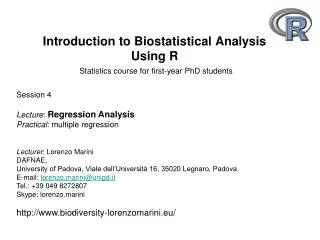
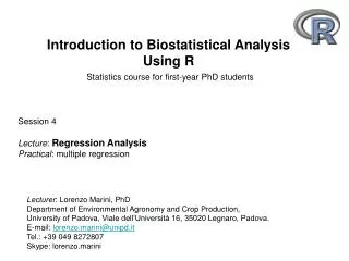
Introduction to Biostatistical AnalysisStatistics course for PhD students in Veterinary Sciences Session 1: Lecture: Basic concepts Session 2: Lecture: Introduction to statistical hypothesis testing Session 3: Lecture: Analysis of Variance Session 4: Lecture: Regression Session 5: Lecture: Synthesis and applications Lecturer: Lorenzo Marini, PhD Department of Environmental Agronomy and Crop Production, University of Padova, E-mail: lorenzo.marini@unipd.it, Tel.: +39 0498272807, Skype: lorenzo.marini http://www.biodiversity-lorenzomarini.eu/
Introduction to Biostatistical AnalysisStatistics course for first-year PhD students inAgricultural, Forest and Veterinary Sciences 5 Sessions: Lecture: theory + Practical: use of R + Assessment (at least three sessions attended) Analysis of an assigned data set and writing a report Your report should consist of the following 2 items: 1. A 1 page R script fully documenting your analysis. 2. A word document presenting the aims, method of analysis, the results, and an interpretation.
Statistics: Definition STATISTICS -Statistical methods can be used to summarize or describe a collection of data; this is called descriptive statistics. -In addition, patterns in the data may be modeled from samples, and then used to draw inferences about the process or population being studied; this is called inferential statistics. • Statistics = Techniques of • Collecting • Analysing • Drawing conclusions from DATA “A mode of thought” will change the way you do science
Statistics: Population and samples Population: is a set of entities of interest (e.g. PhD students, farms, bees, fishes, dogs…) Samples: is a subset of entities randomly drawn from the population Spatial extent Samples Population Statistics answers RESEARCH questions using samples
Statistics: Population and samples Example: Population of PhD students Question: do female students perform better in stats than male students? How to draw samples? Spatial Extent? Population ♂ ♀ Statistics answers RESEARCH questions using samples
Inferential statistics: logics Statistical testing in five steps: 1. Construct a null hypothesis (H0) (RESEARCH QUESTION) E.g. H0: Does Y hormone concentration depend on age? 2. Choose a statistical analysis E.g. Regression between [hormone] and age 3. Collect the data (sampling) E.g. Sampling dogs with different ages 4. Calculate P-value and test statistic Test of our regression model (F-test) 5. Reject/accept (H0) if p is small/large (ANSWER THE QUESTION) Common error Sampling before (1) constructing the hypothesis and (2) choosing the statistical analysis
Strong vs. weak inference Weak inference (Observational) • Many hypotheses • Correlational SEVERAL alternative hypotheses for explaining the process What is a hypothesis? • a statement that is testable • Testable: can be falsified (K. Popper) Strong inference (Experimental) • A clear hypothesis • A specified test ONE clear testable hypothesis
KEEP IN MIND! 1. Clearer is the question, easier is the sampling, simpler is the statistics to be applied 2. If you have blurry and foggy questions and bad design, you will have to apply complex analyses Where are you? Without statistics you cannot write scientific papers (almost)
1. Construct hypotheses: types of variables Which is/are your response variable/s? Object of your research (e.g. animal fitness, yield, healing time, cow milk production…) Which is/are your explanatory variable/s? Variables for explaining your response variable (e.g. age, risk factors, temperature, hormones, fertilization, diet...) Which are your research questions (hypotheses)? HYPOTHESIS: a statement that can be falsified
1. Construct hypotheses Variables Univariate analysis Y - One Response variable (Y): (e.g. Y= Hormone concentration) - One or more explanatory variables (Xi) (e.g. age, size, breed…) Multivariate analysis Y1 Y2 Y3 Y4 Y5 Variables - More than 1 response variable (Yi) (e.g. Yi= Horse exercise parameters) - One or more explanatory variables (xi) (e.g. age, training, breed, sex, )
1. Construct hypotheses Box-plot Scatter plot
2. Choose a statistic analysis Continuous Response variable 1 Univariate Distributions Count Proportion More Multivariate
2. Choose a statistic analysis Response Variable: Distributions Explanatory Variables: Statistical analyses
2. Choose a statistic analysis • Parametric statistics • The population is assumed to fit any parameterized distributions. • A probability distribution describes the values and probabilities that a random event can take place • Normal • Poisson • Gamma • Binomial… General Linear Models (ANOVA, regression, ANCOVA) Generalized Linear Models GLMs NB The distribution depends on the nature of your response variable Non-parametric statistics Nonparametric methods are often referred to as ‘distribution free’ methods as they do not rely on assumptions that the data are drawn from a given probability distributions.
2. Choose a statistic analysis Statistical analysis Assumptions Each analysis (even non-parametric) requires to make some background assumptions Sampling design Each analysis requires an appropriate sampling design If both these conditions are met 5. We can accept/refuse our hypotheses
3. Collect the data (sampling): Population Samples Key step in any research SAMPLING Sampling is that part of statistical practice concerned with the selection of individual observations intended to yield some knowledge about a population of concern Key concepts: -Randomization -Replication (no pseudo-replication!!!) -Independence
3. Collect the data: randomization Population (N) Sample (n<N) 1 2 Without replacement 3 … n A simple random sample is selected so that every possible sample has an equal chance of being drawn from the population Copy and paste in R ###Draw randomly one student among you students<-seq(1,30) ## assign to each student an ID students ##show the ID numbers sample(students,1) ## select randomly one among the 16 hist(replicate(1000,sample(students,1)), breaks=8)
3. Collect the data: randomization Simple randomization is selected so that every possible sample has an equal chance of being drawn from the population Stratified randomization is selected so that every possible sample has an equal chance of being drawn from each stratum of the population Blocked randomization is a random allocation made in blocks in order to keep the sizes of treatment groups similar
3. Collect the data: replication True replication vs. pseudoreplication Replication means having replicate observations at a spatial and temporal scale that matches the application of the experimental treatments True replicates must be independent n replicates Degree of freedom P Replicates MUST NOT: - Come from a time series - Be grouped in space - Be repeated measures on the same individuals (but it depends:wait for mixed models!!!)
3. Collect the data: independence Population 4 replicates Random sampling 4 replicates Independence Intuitively means that the occurrence of one event makes it neither more nor less probable that the other occurs. No meaningful relation between the sampling units 3 MAIN PROBLEMS IN BIOSTATISTICAL ANALYSES 1. Spatial dependence (e.g. spatial autocorrelation) 2. Temporal dependence (e.g. repeated measures) 3. Biological dependence (e.g. siblings)
3. Collect the data: spatial dependence Effect of breed on milk production Farm Cow SH Hurlbert 1984, Ecological Monographs 54, 187-211
3. Collect the data: spatial dependence Which is your replicate and which is the right scale? ♂ ♀ 10 birds per sex 15 feathers per bird 150 measurements 18 rats 18 liver 3 samples per liver 2 analyses per tissue sample 108 measurements
3. Collect the data: spatial dependence Which is your replicate and which is the right scale? ♀ Response variable Feather length Explanatory variable Sex (♀ and ♂) ♂ 15 measures per bird
3. Collect the data: spatial dependence Which is your replicate and which is the right scale? E.g. ANOVA > Bird_level<-aov(feather ~ sex) df SS MS F value P sex 1 3.4279 3.42 5.887 0.025 * Residuals 18 10.4813 0.58 --------------------------------------------------- > Feather_level<-aov(feather ~ sex) df SS MS F value P sex 1 51.41 51.41 63.19 3.9e-14 *** Residuals 298 242.48 0.81 Pseudo-replication!!! Do you have a solution?
3. Collect the data: temporal dependence Temporal dependence: time series (not covered) When we measure experimental units repeatedly over time, we are collecting longitudinal data, also called repeated measures data. Time 1 Time 2 Time 3 Time 4 measure 1 measure 2 measure 3 measure 4
3. Collect the data: biological dependence Biological dependence Unknown genetic relations between sampled units Individuals belonging to same litter or brood Drug A Drug B Litter B Litter A Biased sampling (factor + noise) Proper sampling (2 litter + diet)
3. Collect the data (sampling) If temporal or spatial dependence exists BEST SOLUTION To have an appropriate number of replicates at the proper scale [P.A. Murtaugh 2007. Simplicity and complexity in ecological data analysis. Ecology, 88, 56–62] ALTERNATIVE SOLUTION Wait for mixed models (they can deal with non-independent data) Agricultural research: easy to control possible confounding factors Ecological research: more difficult to apply traditional models. Modern mixed models with REML estimation (extremely dangerous analyses!!!)
3. Collect the data (sampling) ‘Bad’ design no replication (you cannot use statistics) clumped segregation (totally uninformative) isolative segregation (growth chambers etc.) systematic (problem: periodic variations) ‘Good’ Designs randomized block (paired or block design) completely randomized (if enough time, space, money)
3. Collect the data (sampling): one example Factors: Irrigation ------- Response: Maize yield i step: identify your sampling unit ii step: identify your replicate and the sample size iii step: decide the spatial distribution iv step: one or repeated measurements? Arable field Ditch
3. Collect the data (sampling) ‘Good’ design (multifactorial ANOVA) A C D B Latin square (in case of two gradients) D A B C B D C A B A D C Split-plot (very common!) E.g. Agronomic trials, greenhouses, Petri dishes Nested (especially in medicine) E.g. liver samples from individual rat
3. Collect the data (sampling) Before sampling you MUST know which is your REPLICATE and the right SCALE of your study!!! Sampling with appropriate replication!!!
3. Collect the data (sampling) Manipulative experiments Natural experiments Observational studies If we know exactly the analysis the choice of the sampling is straightforward Spatial patterns in the samples If you don’t work with experiments you should always consider the spatial patterns in your sapling design
Basic concepts: mean and variance MEAN AND VARIANCE Whereas the mean is a way to describe the location of a distribution, the variance is a way to capture its scale or degree of being spread out. mean Body size
Basic concepts: Residuals RESIDUALS A residual is an observable estimate of the unobservable statistical error. The simplest case involves a random sample of n men whose heights are measured. residual mean The difference between the height of each man in the sample and the observable sample average is a residual. Residuals represent what we cannot explain
Basic concepts: Uncertainty Population We normally compute means using samples. It is not feasible to measure all the individuals in a population. As we work with samples, there is a degree of UNCERTAINTY in the estimation. Mean=40 Mean=39.5 Mean=42 How can we reduce the degree ofuncertainty?
Basic concepts: Law of the Large Numbers As the sample size (n) grows, the sample mean approaches to the population mean Population with mean = 0 SD = 1 When is a sample large enough? Run the simulation to answer library(animation) ani.options(ani.height = 480, ani.width = 600, outdir = getwd(), nmax =100, interval = 0.1, title = "Demonstration of the Law of Large Numbers", description = "The sample mean approaches to the population mean as the sample size n grows.") ani.start() par(mar = c(3, 3, 1, 0.5), mgp = c(1.5, 0.5, 0)) lln.ani(FUN = rnorm, mu = 0, np = 50, pch = 20, col.poly = "grey") ani.stop()
Basic concepts: Uncertainty Standard error (SE) SE is simply the SD of the probability distribution of a specific statistic. E.g. SE of the mean Confidence intervals (CI) CI is an interval estimate of a population parameter. How likely the interval is to contain the parameter is determined by the confidence level (95%) t distribution (n<30) Normal distribution (n>30)
Basic concepts DEGREE OF FREEDOM The number of INDEPENDENT measurementsminus the number of parameters estimated from the data Df does not correspond to the sum of the single measures but must be computed on our replicates The number of the df define the scale of our analyses!!! Look at the error df to spot pseudo-replication
Basic concepts: Why distributions? We use distribution in statistics mainly in 2 ways: 1. To model our response variables we need to know its distribution (assumptions) 2. Once we know the distribution we can run a statistical test (There are loads of tests to do (F test, t test etc.) No matter what test we do, the principal is always the same: -> Calculate a test statistic (e.g. z, t, F) which follows a DEFINED DISTRIBUTION -> Look up the critical value related to our level of significance -> Compare the calculated value with the critical value ->We can then associate a PROBABILITY to our decision
Basic concepts: Normal distribution Normal standardized (mean=0, sd=1) E.g. Suppose we have measured the heights of 100 people. The mean height was 170 cm and the sd was 8 cm • shorter than a particular height? • taller than a particular height? • between one specified height and another?
Basic concepts: Poisson distribution The Poisson distribution, which describes a very large number of individually unlikely events that happen (count data) Non-negative values Variance=mean Right skewed 1 Parameter: λ (mean=variance) Use: count data Sample from a Poisson distribution (n=1000, mean=variance=0.2) var = mean
Basic concepts: Binomial distribution The binomial distribution describes the number of successes in a finite series of independent Yes/No experiments. 2 Parameters: sample size, probability Use: proportion data and power analysis
What’s R? R is a system for statistical computation and graphics. It consists of a language plus a run-time environment with graphics, a debugger, access to certain system functions, and the ability to run programs stored in script files. R has a home page at http://www.R-project.org/. It is a free software distributed under a GNU-style copyleft, and an official part of the GNU project (“GNU S”).
Why R? The benefits of R are: + R is free. R is open-source and runs on UNIX, Windows and Macintosh + R has an excellent built-in help system + R has excellent graphing capabilities + Students can easily migrate to the commercially supported S-Plus program if commercial software is desired + R's language has a powerful, easy to learn syntax with many built-in statistical functions + The language is easy to extend with user-written functions + R is a computer programming What is R lacking compared to other software solutions? - It has a limited graphical interface (S-Plus has a good one). This means, it can be harder to learn at the outset. - There is no commercial support. (Although one can argue the international mailing list is even better) - The command language is a programming language so students must learn to appreciate syntax issues etc.
Appendix 1 Box-plot explanation