Download
1 / 29
290 likes | 763 Vues
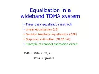
Equalization in a wideband TDMA system. Three basic equalization methods Linear equalization (LE) Decision feedback equalization (DFE) Sequence estimation (MLSE-VA) Example of channel estimation circuit. Three basic equalization methods (1). Linear equalization (LE):.

E N D
Equalization in a wideband TDMA system • Three basic equalization methods • Linear equalization (LE) • Decision feedback equalization (DFE) • Sequence estimation (MLSE-VA) • Example of channel estimation circuit
Three basic equalization methods (1) Linear equalization (LE): Performance is not very good when the frequency response of the frequency selective channel contains deep fades. Zero-forcing algorithm aims to eliminate the intersymbol interference (ISI) at decision time instants (i.e. at the center of the bit/symbol interval). Least-mean-square (LMS) algorithmwill be investigated in greater detail in this presentation. Recursive least-squares (RLS) algorithm offers faster convergence, but is computationally more complex than LMS (since matrix inversion is required).
Three basic equalization methods (2) Decision feedback equalization (DFE): Performance better than LE, due to ISI cancellation of tails of previously received symbols. Decision feedback equalizer structure: Feed-back filter (FBF) Input Output Feed-forward filter (FFF) + + Symbol decision Adjustment of filter coefficients
Three basic equalization methods (3) Maximum Likelihood Sequence Estimation using the Viterbi Algorithm (MLSE-VA): Best performance. Operation of the Viterbi algorithm can be visualized by means of a trellis diagram with mK-1 states, where m is the symbol alphabet size and K is the length of the overall channel impulse response (in samples). State trellis diagram Allowed transition between states State Sample time instants
0 fs = 1/T f Linear equalization, zero-forcing algorithm Basic idea: Raised cosine spectrum Transmitted symbol spectrum Channel frequency response (incl. T & R filters) Equalizer frequency response =
Zero-forcing equalizer Transmitted impulse sequence Communication channel Equalizer Input to decision circuit FIR filter contains 2N+1 coefficients FIR filter contains 2M+1 coefficients Overall channel Channel impulse response Equalizer impulse response Coefficients of equivalent FIR filter (in fact the equivalent FIR filter consists of 2M+1+2N coefficients, but the equalizer can only “handle” 2M+1 equations)
Zero-forcing equalizer We want overall filter response to be non-zero at decision time k = 0 and zero at all other sampling times k 0 : (k = –M) This leads to a set of 2M+1 equations: (k = 0) (k = M)
Minimum Mean Square Error (MMSE) The aim is to minimize: (or depending on the source) Input to decision circuit Estimate of k:th symbol Error + Channel Equalizer
MSE vs. equalizer coefficients quadratic multi-dimensional function of equalizer coefficient values Illustration of case for two real-valued equalizer coefficients(or one complex-valued coefficient) MMSE aim: find minimum value directly (Wiener solution), or use an algorithm that recursively changes the equalizer coefficients in the correct direction (towards the minimum value of J)!
Wiener solution We start with the Wiener-Hopf equations in matrix form: R = correlation matrix (M x M) of received (sampled) signal values p = vector (of length M) indicating cross-correlation between received signal values and estimate of received symbol copt = vector (of length M) consisting of the optimal equalizer coefficient values (We assume here that the equalizer contains M taps, not 2M+1 taps like in other parts of this presentation)
Correlation matrix R & vector p where M samples Before we can perform the stochastical expectation operation, we must know the stochastical properties of the transmitted signal (and of the channel if it is changing). Usually we do not have this information => some non-stochastical algorithm like Least-mean-square (LMS) must be used.
Algorithms Stochastical information (R and p) is available: 1. Direct solution of the Wiener-Hopf equations: 2. Newton’s algorithm (fast iterative algorithm) 3. Method of steepest descent (this iterative algorithm is slow but easier to implement) Inverting a large matrix is difficult! R and p are not available: Use an algorithm that is based on the received signal sequence directly. One such algorithm is Least-Mean-Square (LMS).
Conventional linear equalizer of LMS type Widrow Received complex signal samples Transversal FIR filter with 2M+1 filter taps LMS algorithm for adjustment of tap coefficients T T T + Complex-valued tap coefficients of equalizer filter Estimate of k:th symbol after symbol decision
Joint optimization of coefficients and phase Equalizer filter Coefficient updating Phase synchronization + Godard Proakis, Ed.3, Section 11-5-2 Minimize:
Least-mean-square (LMS) algorithm (derived from “method of steepest descent”) for convergence towards minimum mean square error (MMSE) Real part of n:th coefficient: Imaginary part of n:th coefficient: Phase: Iteration index Step size of iteration equations
LMS algorithm (cont.) After some calculation, the recursion equations are obtained in the form
Effect of iteration step size smaller larger Slow acquisition Poor stability Poor tracking performance Large variation around optimum value
Decision feedback equalizer T T ? + FBF + T T T LMS algorithm for tap coefficient adjustment FFF
Decision feedback equalizer (cont.) The purpose is again to minimize where • Feedforward filter (FFF) is similar to filter in linear equalizer • tap spacing smaller than symbol interval is allowed => fractionally spaced equalizer • => oversampling by a factor of 2 or 4 is common • Feedback filter (FBF) is used for either reducing or canceling (difference: see next slide) samples of previous symbols at decision time instants • tap spacing must be equal to symbol interval
Decision feedback equalizer (cont.) • The coefficients of the feedback filter (FBF) can be obtained in either of two ways: • Recursively (using the LMS algorithm) in a similar fashion as FFF coefficients • By calculation from FFF coefficients and channel coefficients (we achieve exact ISI cancellation in this way, but channel estimation is necessary): Proakis, Ed.3, Section 11-2 Proakis, Ed.3, Section 10-3-1
Channel estimation circuit Proakis, Ed.3, Section 11-3 Estimated symbols Filter length = CIR length T T T LMS algorithm + k:th sample of received signal Estimated channel coefficients
Channel estimation circuit (cont.) • 1. Acquisition phase • Uses “training sequence” • Symbols are known at receiver, . • 2. Tracking phase • Uses estimated symbols (decision directed mode) • Symbol estimates are obtained from the decision circuit (note the delay in the feedback loop!) • Since the estimation circuit is adaptive, time-varying channel coefficients can be tracked to some extent. Alternatively: blind estimation (no training sequence)
Channel estimation circuit in receiver Mandatory for MLSE-VA, optional for DFE Symbol estimates (with errors) Training symbols (no errors) Estimated channel coefficients Channel estimation circuit Equalizer & decision circuit Received signal samples “Clean” output symbols
Theoretical ISI cancellation receiver (extension of DFE, for simulation of matched filter bound) Precursor cancellation of future symbols Postcursor cancellation of previous symbols Filter matched to sampled channel impulse response + If previous and future symbols can be estimated without error (impossible in a practical system), matched filter performance can be achieved.
MLSE-VA receiver structure Matched filter NW filter MLSE (VA) Channel estimation circuit MLSE-VA circuit causes delay of estimated symbol sequence before it is available for channel estimation => channel estimates may be out-of-date (in a fast time-varying channel)
MLSE-VA receiver structure (cont.) The probability of receiving sample sequencey (note: vector form) of length N, conditioned on a certain symbol sequence estimate and overall channel estimate: Since we have AWGN Length of f (k) Objective: find symbol sequence that maximizes this probability This is allowed since noise samples are uncorrelated due to NW (= noise whitening) filter Metric to be minimized (select best .. using VA)
MLSE-VA receiver structure (cont.) We want to choose that symbol sequence estimate and overall channel estimate which maximizes the conditional probability. Since product of exponentials <=> sum of exponents, the metric to be minimized is a sum expression. If the length of the overall channel impulse response in samples (or channel coefficients) is K, in other words the time span of the channel is (K-1)T, the next step is to construct a state trellis where a state is defined as a certain combination of K-1 previous symbols causing ISI on the k:th symbol. Note: this is overall CIR, including response of matched filter and NW filter 0 K-1 k
MLSE-VA receiver structure (cont.) At adjacent time instants, the symbol sequences causing ISI are correlated. As an example (m=2, K=5): : At time k-3 1 0 0 1 0 At time k-2 1 0 0 1 0 0 At time k-1 1 0 0 1 0 0 1 At time k 1 0 0 1 0 0 1 1 : 16 states Bit detected at time instant Bits causing ISI not causing ISI at time instant
MLSE-VA receiver structure (cont.) State trellis diagram Number of states The ”best” state sequence is estimated by means of Viterbi algorithm (VA) Alphabet size k-3 k-2 k-1 k k+1 Of the transitions terminating in a certain state at a certain time instant, the VA selects the transition associated with highest accumulated probability (up to that time instant) for further processing. Proakis, Ed.3, Section 10-1-3