Download
1 / 34
400 likes | 708 Vues
The Antarctic Circumpolar Current (ACC). Richard Karsten Acadia University. The ACC. Around Antarctica, there is an open patch of ocean that stretches all the way around the globe. It is the only such stretch of ocean on earth. The ACC.

E N D
The Antarctic Circumpolar Current(ACC) Richard Karsten Acadia University
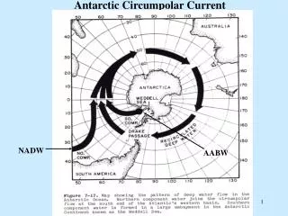
The ACC Around Antarctica, there is an open patch of ocean that stretches all the way around the globe. It is the only such stretch of ocean on earth.
The ACC This open patch of ocean allows an eastward current, the Antarctic Circumpolar Current or ACC, to flow around the globe. It is the worlds largest current, carrying 130 times the volume of water of all the world’s rivers combined Here we’ve shown the path of the current estimated using satellite altimetry data.
The ACC directly effects the climate of Antarctica, which has been in the news a lot lately. The different stories make it clear that we need to understand this region better. Antarctic Ice Shelf Collapses “… attributed to a strong climate warming in the region …[at a] rate of … approximately 0.5 degrees Celsius per decade …” Antarctic climate cooling and terrestrial ecosystem response PETER T. DORAN*, et al. * “… a net cooling on the Antarctic continent … cooled by 0.7°C per decade between 1986 and 2000 …” Why is the ACC important?
S Mean density N Thermal wind Structure of the ACC We can start to understand the ACC by looking at a cross section of it. Using hydrographic data collected by ships over the past century, we can plot the average density and velocity of the ACC
wind stress: The roaring forties and furious fifties! The ACC is driven by strong westerly winds, the strongest winds in the world. Here we show the stress the wind applies to the ocean estimated from ship measurements. The arrows indicate the direction and strength.
along-stream mean The roaring forties and furious fifties! If we average the winds along streamlines, we see the winds are a maximum in the region of circumpolar flow as marked by the red bars.
S N Winds and Ekman Transport Because of the rotation of the earth, the westerly winds drive an overturning circulation, which draws fluid up in polar waters, pulls it Northward at the surface and then pumps in downward in the subtropics This overturning can be described by a mean streamfunction, which also gives the Ekman transport. The net effect of winds is to transport, warm and light surface waters out of the polar region.
Altimetry GFDL simulation Eddy Fluxes What could balance the effect of the winds? The answer becomes obvious when we look at snap shots of the ACC using either satellite observations (top) or numerical simulations (bottom). The ACC is not a steady current, but is made of constantly evolving waves and eddies. When averaged over time, these eddies produce the flow we call the ACC. The heat transport associated with the eddies can be described with the eddy-induced streamfunction above. Calculating this quantity gives a southward transport.
A balance between winds and eddies This allows for a basic balance between the winds and the eddies: the winds transport heat northwards and the eddies transport it southward. We might postulate that the sum of the two streamfunctions vanishes.
We introduce the Residual Circulation, the sum of our two streamfunctions. Mathematically • We begin by considering the mean buoyancy equation: • This gives us Transformed Eulerian mean equation, which states that the residual circulation is driven by the forcing. If forcing is weak, then the residual circulation vanishes.
(winds) S N (eddies) estimated from altimetry What does this balance actually look like? Using satellite and hydrographic data, we calculate the two streamfunctions and plot them above. The winds and eddies do oppose each other and produce a weak residual transport. Note that the residual circulation changes sign at the center of the ACC. This is the Antacrtic Convergence, where northward moving flow meets southward moving flow.
Momentum balance: above topography • We can also examine this balance using the momentum equations to get a balance between the momentum the winds put in and eddy form stress as follows: • Transformed Eulerian momentum equation: Integrate over depth h: (assume residual circulation is weak)
W E H L What about topography? The ACC flows over large topography as shown in the figure. This allows the momentum input by the winds to be balance by bottom form drag. As the flow goes over topography, it creates high pressure upstream and low pressure downstream. Note the ACC deflects northward as it passes over topography.
H L H L Momentum balance: with topography W E • Mean along-stream momentum: Between two topographic features, we get a pressure gradient. This gradient produces a force, bottom drag, which balances the winds as follows. Integrate over depth h:
Support from numerical modelsOlbers and Ivchenko 2002 When the various terms are plotted versus depth, we see the initial balance between eddies and winds, becomes a balance between winds and bottom drag. (at least in the region of circumpolar flow, middle) This balances has been illustrated in numerical simulations, which illustrate the balance of winds and bottom drag at all latitudes.
Barotropic: What determines the path of the ACC? There are several theories of what determines the path of the ACC. One theory is the ACC is barotropic, that is it acts like a single layer of homogeneous fluid. The streamlines would then be given by the geostrophic contours f/H. Here we’ve plotted these contours with the colours (red high values, blue low). If the theory was accurate, the path of the ACC given in black would not cross contours of different colours. Obviously the theory does not hold well. The ACC is not barotropic.
Strongly Baroclinic: (no topography) What determines the path of the ACC? A second theory assumes the ACC is strongly baroclinic and does not feel topography, and so just follows lines of constant latitude. Again, we’ve plotted these contours and it is clear that the ACC crosses contours of different colours.
Variations in topography are small: Something in between? A more promising theory, is something in between these two, where topography is weak but not negligible. This gives the streamlines above. If we choose H0 to be the average depth of the ocean, we get the picture to the right, better but not great.
Variations in topography are small: Something in between? However, if we use more knowledge of the stratification and choose H0 to be a much larger value, we get a new picture that begins to look reasonable. We need to know the stratification if we want to know how topography affects the path of the ACC (Killworth and Hughes 2002)
Exponential profile: Our laboratory (top) and numerical simulations (bottom) have suggested that the stratification may have a simple vertical structure, an exponential function given at the top of the page. Lab and numerical experiments
Observations (2% error) Exponential profile: If we try to fit this simple curve to hydrographic data, we find that there is also extremely good agreement. In the graph the blue curve is the data, the red curve is the best-fit exponential. The error is extremely small.
Error in Exponential Profile If we repeat this procedure at each longitude-latitude grid point in the Southern Ocean, an amazing pattern reveals itself. Here we’ve plotted the error in fitting the curve. We see that the error is very small (blue) in a circumpolar region that agrees almost exactly with the path of the ACC (black curves).
E-folding depth Here we’ve plotted the e-folding depth at all grid points. It is clear that it is not constant but varies from low values in polar waters to high values in the subtropics. It looks like it might be constant along streamlines of the ACC.
E-folding depth If we plot the contours of the e-folding depth, we get what might be reasonable streamlines of the ACC. So, understanding the ACC seems intricately tied to understanding the vertical stratification.
formula formula with he Predicting the Depth(Karsten and Marshall, DAO 2002) We have begun to tie the balance of winds and eddies to predicting the stratification, as summarized below.
Measuring eddies from satellites An important aspect of many of our results is determining the eddy fluxes. We do so by estimating the eddy diffusivity from satellite altimetry. This diffusivity is plotted here and highlights the fact that the ACC is region of high eddy activity
Climate and surface fluxes Finally, we return to the idea of the residual circulation. Examining our mathematics, we can connect the residual circulation to surface fluxes and diffusion. • Transformed Eulerian mean: (Andrews and McIntyre, 1976) Integrate over mixed layer: In the interior:
S N H B Q Buoyancy Flux Using our calculated residual circulation, we can estimate the surface buoyancy fluxes as shown. They suggest a large buoyancy gain near the southern boundary of the ACC. If we decompose the surface flux into heat (blue) and freshwater (green) fluxes, we see that the majority of the buoyancy gain is due to heat fluxes.
Comparing to Speer et al. (2000) analysis of COADS data S N Buoyancy Flux We have compared our estimated fluxes (blue curves) to analysis of observed fluxes (red curve). The excellent agreement between two different approaches suggests we’re making progress.
buoyancy buoyancy SAMW S N 24 Sv AAIW UCDW Full Residual Circulation It also helps us describe the transformation of water masses. For example, deep water rises to the surface south of the ACC, gains buoyancy as it moves northward and the sinks to form intermediate water We can also calculate the full residual circulation (red and blue lines). This clearly illustrates the overturning structure of the ACC and the Antarctic convergence in the center of the ACC.
S S N N Tracer Transport Dissolved Oxygen Salinity As a test of our calculations, we compare the residual circulation we calculate to the distribution of two tracers, salinity and dissolved oxygen, which we’ve plotted here.
Salinity S S N N Tracer Transport Dissolved Oxygen When we overlay the contours of our residual circulation, we see a remarkable agreement in the patterns. Again, this is an indication that we are making progress.
Conclusions • The ACC is all about eddies • eddy transport balances Ekman transport • eddy form-stress transfers wind momentum down to topography • eddies play key role in determining stratification, which determines path of ACC • the balance of eddies and winds determine the residual circulation which in turn can be used to diagnose surface buoyancy fluxes and tracer distribution Preprints http://ace.acadiau.ca/math/Karsten/publications.html