Response Surface Methodology
Response Surface Methodology. Introduction. Main Part I (General Concept). Main Part II (Advanced RSM). Ending. Contents. Basic Concept, Definition, & History of RSM Introduction ; Motivation. DOE (Design Of Experiments) Experiments (Numerical) & Databases


Response Surface Methodology
E N D
Presentation Transcript
Response Surface Methodology Intelligent System Design Lab.
Introduction Main Part I (General Concept) Main Part II (Advanced RSM) Ending Contents • Basic Concept, Definition, & History of RSM • Introduction ; Motivation • DOE (Design Of Experiments) • Experiments (Numerical) & Databases • Construction of RSM (Response Surface Model) • Optimization Using RS Model (Meta Model) • Examples • Efficient RS Modeling Using MLSM and Sensitivity • Design Optimization Using RSM and Sensitivity • Conclusion • Further Study Intelligent System Design Lab.
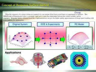
1.1 Concept of Response Surface Method Input Response Black Boxed System DOE and Experiments RS Model 1 0 x2 -1 0 1 -1 x1 Original System RSM : Response Surface Method : Response Surface Model Intelligent System Design Lab.
1.2 Definition of Response Surface Method Box G.E.P. and Draper N.R.,1987 A simple function, such as linear or quadratic polynomial, fitted to the data obtained from the experiments is called a response surface, and the approach is called the response surface method. Myers R.H., 1995 Response surface method is a collection of statistical and mathematical techniques useful for developing, improving, and optimizing processes. Roux W.J.,1998 Response surface method is a method for constructing global approximations to system behavior based on results calculated at various points in the design space. Intelligent System Design Lab.
1.3 History of Response Surface Method Research of DOE 1951 Box and Wilson - CCD 1959 Kiefer - Start of D-optimal Design 1960 Box and Behnken - Box-Behnken deign 1971 Box and Draper - D-optimal Design 1972 Fedorov - exchange algorithm 1974 Mitchell - D-optimal Design Application in Optimization 1996 Burgee - design HSCT 1997 Ragon and Haftka - optimization of large wing structure 1998 Koch, Mavris, and Mistree - multi-level approximation 1999 Choi / Mavris – Robut, Reliablity-Based Design App in Optimization & Reduce the Approximation Error Intelligent System Design Lab.
1.4 Introduction - Motivation of RSM Heavy Computation Problem Approximation When Sensitivity is NOT Available Global Behavior Real / Numerical Experiment When the Batch Run is Impossible For Any System Which has Inputs and Responses Easy to Implement Part of MDO, Concurrent Engineering Probabilistic Concept Noisy Responses or Environments Advantages Approximation Error Size of the Approx. Domain is Very Dominant Disadvantages Intelligent System Design Lab.
Part I(Classical RSM) Intelligent System Design Lab.
DOE (Design Of Experiments) Experiments (Numerical) & Databases Construction of RSM (Response Surface Model) Optimization Using RS Model (Meta Model) Intelligent System Design Lab.
2.1 DOE 1 – Factorial Design Classifications - 2 / 3 level Factorial Design - Full / Fractional Factorial Design 2 level Full Factorial Design Fractional Factorial Design Intelligent System Design Lab.
2.1 DOE 2 – Central Composite Design(CCD) Characteristics 3 DV Quadratic RS Model Effective than Full-Factorial Design Rotatability Factorial Points 2 DV 1 Axial Points 0 x2 -1 0 1 Center Points x1 Intelligent System Design Lab.
2.1 DOE 3 – Box-Behnken Design Treatment X1 X2 X3 Block1 0 Block2 0 Block3 0 Characteristics Quadratic RS Model Effective 3 Level Design Balanced Incomplete Block Design Block1 Block2 Block3 Center Point Intelligent System Design Lab.
2.1 DOE 4 – D-Optimal Design vector of the observations matrix of the level of the independent variables vector of the regression coefficients vector of random errors Characteristics The Most Popular DOE Arbitrary Number of Experiment Points Possible to Add Points Specified Functional Form of the Response Approximation Function (RSM) Coefficients of RSM Variance of Coefficients Good fitting Intelligent System Design Lab.
2.1 DOE 5 – Latin-Hypercube Design Characteristics Arbitrary Number of Experiment Points No Priori Knowledge of the Functional Form of the Response Initial Information No. of Variables : k No. of Experiments : n Main Principles 1. No. of Levels = No. of Experiments 2. Experiment points in the design space are distributed as regular as possible. Intelligent System Design Lab.
DOE (Design Of Experiments) Experiments (Numerical) & Databases Construction of RSM (Response Surface Model) Optimization Using RS Model (Meta Model) Intelligent System Design Lab.
2.2 Experiments (Numerical) & Databases Input Response Black Boxed System(FE Model) *.bdf *.cdb *.f06 , *.pch *.rst NASTRAN ANSYS Rewrite Input Files Read Output Files Intelligent System Design Lab.
DOE (Design Of Experiments) Experiments (Numerical) & Databases Construction of RSM (Response Surface Model) Optimization Using RS Model (Meta Model) Intelligent System Design Lab.
2.3 Construction of RSM – Least Squares Method LSM Original Response RSM Response Optimum By RSM Approximation Error True optimum Response • - Global Approximation • 1 RS Function at all pts • Constant Coefficients Input Intelligent System Design Lab.
2.3 Construction of RSM – Least Squares Method(’) vector of the observations matrix of the level of the independent variables vector of the regression coefficients vector of random errors - 1. Approximation Function (RSM) - 2. Least Squares Function DOE - 3. Minimize Least Squares Function - 4. The coefficients of the RS model Intelligent System Design Lab.
2.3 Example – Construction Of RSM Original Function Number of Design Variable = 2 Number of Experiment(FFD) = 9 RS Model = Quadratic Model RSM Function JMP, SAS, SPSS MATLAB Statistics Toolbox Visual-DOC In-House Codes Software Intelligent System Design Lab.
2.3 Construction of RSM – Test Criteria : The level of significance, generally 0.01 or 0.05 K : Degree of freedom of regression n-k-1 : Degree of freedom of error or residual F-Test (ANOVA) The model was fitted well. Intelligent System Design Lab.
2.3 Construction of RSM – Test Criteria (Continued) The coefficient of determination 1.0 Adjusted R2 1.0 t-Test Where Cjj diagonal term in (X’X)-1 corresponding to bj xjis a dominant term of RS model Prediction Test Intelligent System Design Lab.
2.3 Construction of RSM – Variable Selection Concept Unnecessary Term Original System RS Model All Possible Regression Minimize Stepwise Regression • Forward regression • Backward regression • Stepwise regression (Backward + Forward ) Intelligent System Design Lab.
DOE (Design Of Experiments) Experiments (Numerical) & Databases Construction of RSM (Response Surface Model) Optimization Using RS Model (Meta Model) Intelligent System Design Lab.
2.4 Optimization Using RSM - Whole Sequences Sensitivity Analysis Sensitivity If RSM using Sensitivity Reliable RSM ? No Test Criteria Yes Optimizer No 1 Analysis at opt from RSM Reliable OPT? Calc Error Yes Optimization Problem Variable Selection Approximation Domain DOE & Experiments Construct RSM Optimization Using RSM Estimated Opt Response Final Optimal Solution Intelligent System Design Lab.
2.5 Example 1 – System / Problem Setup Problem Setup System(FE Model) Min : weight s.t : Initial variables Intelligent System Design Lab.
2.5 Example 1 – Optimization Using RSM Constructed RSMs DOE & Experiments Xl <= X <= Xu 0.001 <= X <= 0.0021 DOE ( CCD=15 ) & Analysis Optimization Results Optimization Min : Obj_func s.t. constraint 1 constraint 2 constraint 3 Intelligent System Design Lab.
2.5 Example 2 - Induction Motor FE Model Update Real System Model : WM0F3A-S Induction motor LMS CADA-X Upper Housing Stator Lower Housing Rotor Reliable FE Model ?? (close to Real Model ) FE Model (NASTRAN) Intelligent System Design Lab.
2.5 Example 2 - Modal Analysis(1/2) Upper Housing Lower Housing 1 2 1 2 Rotor Stator 1 2 2 1 Intelligent System Design Lab.
2.5 Example 2 - Model Update Using RSM : Rotor Accumulated Material DOE and Analyses Using RSM Design Variables D-optimal Design 22 times of analyses 4 D.V. Optimization Construct RS Model For Each Frequencies Frequency 1 = F1(x) Frequency 2 = F2(x) Optimizer : DOT Intelligent System Design Lab.
2.5 Example 2- Model Update Using RSM: Other Parts Upper Housing 5 Design Variables D-optimal Design 29 times of analyses 2 Design Variables CCD Design 9 times of analyses 4 Design Variables D-optimal Design 22 times of analyses Lower Housing Stator Accumulated Material Intelligent System Design Lab.
2.5 Example 2 - Model Assemble & Analysis Mode Shape Natural Frequencies 1 2 3 4 These good Results are from the good part models Sensitivities of all design variables w.r.t. the each frequencies 5 Design Variables are selected Intelligent System Design Lab.
2.5 Example 2 - Model Update : Whole Motor Reliability of RS_Model Reliability of FE_Model Optimization • Gradient-based Optimization • Hybrid(RSM+GRAD) Optimization Final Results – Using Hybrid Method Intelligent System Design Lab.
2.5 Example 3 - AUTOMOTIVE SIDE IMPACT Example by k.k.choi, U. of Iowa, “Moving Least Square Method for Reliability-Based Design Optimization”, WCSMO4, 2001 Intelligent System Design Lab.
References Myers, R. H., and Montgomery, D. C. Response Surface Methodology : Process and Product Optimization Using Designed Experiments. John Wiley & Sons. Inc., New York, 1995 박성현, 회귀분석, 민영사, 1998 박성현, 현대실험계획법, 민영사, 1996 김좌일, “Efficient Response Surface Modeling and Design Optimization Using Sensitivity”, 석사학위 논문, 광주과학기술원, 2001 Nguyen, N. K., and Miller, F. L. “A Review of Some Exchange Algorithms for Constructing discrete D-optimal Designs”, Computational Statistics & Data Analysis, 14, 1992, pp.489-49 Intelligent System Design Lab.
Part II(Advanced RSM) Intelligent System Design Lab.
3.1 Introduction-Motivation Function Test Efficient Construction of RSM using Sensitivity Reduce Approximation Errors Local & Global Approximation (MLSM) Reduce the Computation Time Effect of Function & Sensitivity Restriction -Available Cheap Sensitivity Optimization using RSM and Sensitivity-based Method Induction Motor FE Model Update RSM Optimization Global Behavior / Large Approximation Error Sensitivity-based Optimization Accurate & Fast Convergence / local Behavior Intelligent System Design Lab.
3.2 Moving Least Squares Method LSM MLSM Calculation Point Calculation Point Response • - Global Approximation • 1 RS Function at all pts • Constant Coefficients Input Response • Local Approximation • 1 RS Function at 1 pt • Various Coefficients Input Intelligent System Design Lab.
3.2 Numerical Derivation (1/2) – Moving Least Squares Method vector of the observations matrix of the level of the independent variables vector of the regression coefficients vector of random errors - Response Function - Least Squares Function - The coefficients of the RS model Function of location x Intelligent System Design Lab.
3.2 Numerical Derivation (2/2) – MLSM with Sensitivity the vector of gradient of the response with respect to xj, the transformation matrix which represents gradient vector vector of gradient errors. - Gradient Function - New Least Squares Function - The coefficients of the RS model Intelligent System Design Lab.
3.2 Numerical Examples (Graphical Analysis) RSM 16 Points Experiment 100 Points Test Rosenbrock Function • Function Characteristics • Banana Function • V-shaped Valley Basis Model : Quadratic Weight Function of Resp : 4th order polynomials Weight Function of Grad : 4th order polynomials Intelligent System Design Lab.
3.2 Numerical Examples (Error Analysis) 2 2 1 3 2 3 1 • Response Error • Gradient Error • Global Error Compare & • Response Error • Gradient Error • Global Error Compare & SSE/n = Sum of Squared Errors / No of Sampling Pts SSE/nt = Sum of Squared Errors / No of Test Pts Error Table Resp Error Grad Error Global Error Intelligent System Design Lab.
3.2 Numerical Examples (Graphical Analysis) RSM 16 Points Experiment 100 Points Test 2D six-hump camel back function Basis Model : Quadratic Weight Function of Resp : 4th order polynomials Weight Function of Grad : Exponential 4 local optimums and 2 global optimums within the bounded region Intelligent System Design Lab.
3.2 Numerical Examples (Error Analysis) 1 2 1 3 2 3 2 Sampled 16 points Satisfy a Quadratic Func Compare & • Response Error • Gradient Error • Global Error Compare & SSE/n = Sum of Squared Errors / No of Sampling Pts SSE/nt = Sum of Squared Errors / No of Test Pts Error Table Resp Error Grad Error Global Error Intelligent System Design Lab.
3.2 Numerical Examples (Efficiency Test) MLSM only MLSM with Sensitivity – Narrowed Domain Original Func RSM Func 9 pts Sampling MLSM with Sensitivity Intelligent System Design Lab.
3.3Concept of Hybrid Optimization of RSM & gradient-based optimization Using Response Surface Method Hybrid Optimization (Function Plot) Original Response Use the approximated Function instead of the original system RSM Response Optimum By RSM • (Adv) Global Behavior • (Dis) Large Approximation Error True Optimum by Gradient-based optimization Using Gradient-Based Method Hybrid Optimization (Contour Plot) Search the direction s.t. improve the objective Use the original system • (Adv) Accurate & Fast Convergence • (Dis) local Behavior Intelligent System Design Lab.
3.3 Sequences of the optimization Optimization Problem Variable Selection Sensitivity Approximation Domain Analysis DOE & Experiments Sensitivity If RSM using Sensitivity Construct RSM Reliable RSM ? No Test Criteria Yes Optimization Using RSM Optimizer Estimated Opt Response No 1 Analysis at opt from RSM Reliable OPT? Shift Criteria Analysis Yes Sensitivity Gradient Based Optimization Final Optimal Solution Intelligent System Design Lab.
3.3 Numerical Example Optimizer : DOT Method : SLP/BFGS 1. Gradient Based Optimization 4. Comparison of Results 2. Optimization Using Sequential RSM Local Optimum Too many Computations 3. Optimization Using RSM & Sensitivity (Hybrid) Best Performance Optimization Problem Intelligent System Design Lab.
3.4 Conclusion Efficient Construction of RSM using Sensitivity Local & Global Approximation (MLSM) Reduce the Approximation Errors Function Tests Accuracy & Efficiency Effect of Function & Sensitivity Reduce the Calculation Time Optimization using RSM and Sensitivity-based Method RSM Optimization Global Behavior Function Test & Induction Motor FE Model Update Sensitivity-based Optimization Accurate & Fast Convergence Intelligent System Design Lab.
3.4 Further Study • Apply to Real Optimization Problems Using these Methods • Reliability-Based Design Optimization Using This RSM • Proper Selection of The Weight Factor of Gradient Error (SWg) • Use of Design Of Experiments Intelligent System Design Lab.
3.5 Other Approximation Methods Kriging Model Neural Network Intelligent System Design Lab.