Download
1 / 67
670 likes | 692 Vues
This presentation provides an overview of the preliminary cumulative risk assessment for organophosphorus pesticides, including the historical perspective, milestones, and methodologies used. The presentation also includes key recommendations from the FIFRA Scientific Advisory Panel.

E N D
Preliminary Cumulative Risk Assessment: Organophosphorus Pesticides Presentation to the FIFRA Scientific Advisory Panel U.S. Environmental Protection Agency Office of Pesticide Programs February 5 to 8, 2002
Introduction and Welcome Marcia Mulkey, Director Office of Pesticide Programs
Historical Perspective and Agenda Margaret J. Stasikowski, Director Health Effects Division Office of Pesticide Programs
Where We’ve Been: Milestones Common Mechanism Guidance January 1999 Final Aggregate Guidance November 2001 Draft OP Risk Assessment December 2001 Final Cumulative Guidance January 2002 Final OP Risk Assessment June 2002
March 1997.Common Mechanism Guidance March 1998. OP Common Mechanism of Toxicity September 2000. Endpoints and RPF’s: A Pilot Study September 2001. Preliminary Hazard and Dose-Response How We Got There: SAP Advice Dose-Response and Hazard
September 1997.Residential Scenarios December 1997. Drinking Water March 1998. Probabilistic for Dietary, Residential, and Common Mechanism July 1998. Estimating Pesticide Concentrations in Drinking Water May 1999. Statistical Methods for Acute Dietary and Drinking Water How We Got There: SAP Advice Exposure Assessment September 1999. Residential March 2000. Models for Dietary and Drinking Water June 2000. Drinking Water Survey September 2000. Residential and Dietary Models and Drinking Water March 2001. Dietary Model
March 1997.Aggregate Methodology March 1998. Probabilistic Risk Assessment Methodology February 1999. Aggregate Guidance September 1999. Cumulative and Aggregate Methodology December 1999. Cumulative Methodology September 2000. Risk Assessment Models December 2000. Case Study of 24 OP’s and Cumulative Assessment Methodology How We Got There: SAP Advice Assessment Methodology and Other
Hazard Dose-Response Dietary Key SAP Recommendations • Dose-response modeling: use of exponential model and several other recommendations • Use of PDP and other monitoring data • Use of publicly-available databases and recipes • Finer division of age groups: • New CSFII have more data for children
Drinking Water Key SAP Recommendations • Devote resources to surface water impacts, define higher assessment tiers and develop techniques for estimating concentration distributions for probabilistic risk assessments • Regional modeling • Shift focus to monitoring programs to support model development and evaluation
Residential and Non-occupational Key SAP Recommendations • Hand-to-mouth variables • Use of uniform distribution
Next Steps • Revise December 2001 Preliminary Organophosphate Risk Assessment based on: • This week’s advice from the Panel; • Comments received during the 90-day public comment period • Intended completion date: June 2002
SESSION 1: Hazard Dose-Response SESSION 2: Dietary SESSION 3: Drinking Water SESSION 4: Residential and Non-occupational SESSION 5: Risk Characterization This Week…
Participants Kevin Costello, MA Geology Princeton University Vicki Dellarco, Ph.D. Genetics Iowa State University Elizabeth Doyle, Ph.D. Toxicology American University Jeff Evans, BS Agronomy Delaware Valley College Anna B. Lowit, Ph.D. Environmental Toxicology University of Tennessee
Participants David Miller, MS and MPH Environmental Science Engineering Virginia Tech Environmental Chemistry University of Michigan Randolph Perfetti, Ph.D. Chemistry Virginia Tech R. Woodrow Setzer, Ph.D. Population Biology State University of New York at Stony Brook William O. Smith, Ph.D. Plant Physiology University of Kentucky Nelson Thurman, MS Soil Science West Virginia University
Organization of Presentation • Introduction & Background • Anna Lowit, Ph.D., OPP • Methods: Oral Toxic Potency Determination and Points of Departure • R. Woodrow Setzer, Ph.D., ORD
Introduction & Background Anna B. Lowit, Ph.D. Toxicologist Health Effects Division Office of Pesticide Programs
Nerve Axon Identifying a Common Mechanism: Organophosphate Pesticides Inhibition of Acetyl Cholinesterase • Brain • Peripheral Nervous System (e.g., diaphragm, muscles) • Surrogate (RBC, Plasma) • U.S. EPA 1999 Policy Paper
Timeline of Methodology Development • Pilot Hazard & Dose-Response OP Case Study • Presented to SAP in September 2000 • Preliminary Hazard & Dose-Response: July 2001 document • Presented to SAP in September 2001 • Revised Preliminary Hazard & Dose-Response: December 2001 document
OPs Considered in Hazard & Dose-Response Assessment • 29 Organophosphate Pesticides • Exposure through food, water, and/or residential • Determination of relative potency of chlorethoxyphos, profenofos, and phostebupirim is on-going
Relative Potency Factor Method • Relative toxic potency of each chemical was calculated in comparison to “index chemical” • Exposure equivalents of index chemical are combined in the cumulative risk assessment
Toxicity Data Used • Oral, Dermal, and Inhalation Routes: • Sub-chronic and chronic toxicity studies collected • Same studies were used in July and December 2001 documents • Electronic dataset of oral ChE data is available to the public at: http://www.epa.gov/pesticides/cumulative/EPA_approach_methods.htm
Key Refinements to Hazard and Dose-Response Assessment • Relative potency factors used in Preliminary Cumulative Risk Assessment • Method for combining ChE data • Modeling of low dose region • Measure used in potency determination
RPFs Used in Preliminary CRA • Male RBC RPFs were proposed in July 2001 document • RBC selected primarily on availability of large database and ability to consider time course information • Males selected
RPFs Used in Preliminary CRA • Female Brain RPFs were selected in December 2001 document • Why Brain? • Compared to RBC, tighter confidence limits on potency estimates were observed • Target tissue • Why Female? • Sexes equally sensitive for most • Female rats more sensitive for ~5 OPs
Key Refinements to Hazard and Dose-Response Assessment • Relative potency factors used in Preliminary Cumulative Risk Assessment • Method for combining ChE data • Modeling of low dose region • Measure used in potency determination
Methods: Oral Toxic Potency Determination and Points of Departure R.Woodrow Setzer, Ph.D. Mathematical Statistician National Health and Environmental Effects Laboratory Office of Research and Development
Overview • Review the methods used in July draft of hazard and dose-response assessment chapter. • What issues raised in September SAP report will be addressed here? • How have those issues been addressed? • What have we done since release of the December document?
SAP Report, September 2001 • Overall, SAP was supportive of the approach used by the Agency • Exponential model • Multiple studies and time points • R software for statistical analysis. • Recommended further exploration of dose-response modeling issues which could impact the low dose region. • Comprehensive list described in appendix of preliminary CRA (III.B.3) and can be found at http://www.epa.gov/pesticides/cumulative/.
July: Estimate of Potency and DR 2000 1500 AChE Activity 1000 500 potency 0 0 500 1000 1500 Dose
Potency MRID 1 MRID 2 MRID 3 July: Combining Estimates Fit a model to each dataset, estimating BMD (and estimated standard error) for each dataset. Use the global two-stage method (Davidian and Giltinan, 1995; 138-142) twice, once for each level of variability.
July: Estimating Parameters • Use generalized least squares and assume constant coefficient of variation • Sequential approach to fitting: • Fit full model to all data • If no convergence or inadequate fit, • Repeat (until good fit or # remaining doses < 3): • set B0 • refit to dataset • drop highest dose
Issues from the September SAP Report: • The approach to estimating B could result in biased estimates of m (the potency measure). • The weight function underestimated the variance at low doses and overestimated it at high doses. • The dose response curves for some chemicals appeared to have a “low dose shoulder,” which the basic exponential model did not capture.
Updates to Methods • Change the way models are expressed in terms of the parameters (same model, different parameters). • Use 1/BMD as measure of potency instead of m. • Use nonlinear mixed effects method to fit model to combined data.
Updates to Methods (continued) • Use profile likelihood to estimate a value of B consistent with the data when the standard approach does not converge. • Develop a model for low-dose shape that was inspired by saturable metabolic clearance. • Weights are proportional to means (instead of squares of means).
Model Parameterization July model (for comparison) • December model (factoring out A and replacing B/A with PB )
Model Parameterization (cont.) • Current model (same shape, but in terms of BMD instead of m): Here BMR is the benchmark response (say, a 10% reduction in mean AChE activity), and BMD is the corresponding benchmark dose.
Model Parameterization (cont.) • Advantages of current model: • More stable estimation, since BMD and PB are relatively less correlated than were m and PB. • Simplifies computation of BMD and its standard error.
Model Parametrization (cont.) • Parameters actually estimated: • lA=ln(A) • lBMD=ln(BMD) • B=ln(PB/(1-PB)) • Mainly, to assure legal parameter values (for example, A and BMD>0, 0<PB<1)
Model Fitting • Use nonlinear mixed effects models (nlme in R): • Estimate a separate mean value for lA for each sex X unit combination, and a separate value of B and lBMD for each sex. • Estimate a random effect for each parameter for each level of nesting: maximum of among studies and among datasets within studies.
Model Fitting (cont.) • Weights based on error variances proportional to means.
Model Fitting (cont.) • Sometimes nlme failed to converge to estimates for this full model. Then try (in order:) • Full model (Sex-specific values for B, random effects) • Single value for B, with random effects • Sex-specific values for B, no random effects • Single value for B, no random effects • Fix sex-specific values for B that are consistent with the data, and estimate other parameters given the sex-specific values
Model Fitting (cont.) • Select PB for males and females by choosing the value that maximizes the profile likelihood: • Likelihood (more usually, its natural logarithm, the log likelihood) is a measure of the degree to which the data support a particular parameter value. • Profile likelihood for a parameter (or parameters) results when the parameters in question are fixed, and the remaining parameters estimated given those values (so, fix PB, and estimate A and BMD). The log likelihood of the resulting fit is plotted versus the parameter values. The data most support the parameter value associated with the maximum.
Model Fitting (cont.) • Profile Likelihood (cont.) • PB (males and females) were fixed in turn to each point on an 11 X 11 grid from 0.001 to 0.999. • Log likelihood plotted for each grid point (to aid visualization, values were linearly interpolated between grid points). • The grid point with the largest log likelihood was selected as the value of PB.
Model Fitting (cont.) • Bright yellow (highest value) to Red (lowest value) • Circles: points not significantly different (P>0.05) from best point (likelihood ratio test) • Plus signs (P<0.05)
Model Fitting (cont.) • Sensitivity: How much does the choice of B effect the estimate of the BMD? Only relevant when we cannot estimate PB with the other parameters. • For the same grid of values for PB, plot BMD as a fraction of the value at the selected point. • Plot contours (in the figures, the smallest contour represents ±25%).
The D-R Shape at Low Doses • Some of the data look as if there were a shoulder at the low-dose end of the dose-response. • A proposed explanation is saturable metabolic clearance. • Add a submodel, inspired by this mechanism, to the basic model already described, to create a low-dose shoulder. • Keep it simple!
Qb Body (Cb) Venous Arterial Urine (ke) Ingestion (Dose ×BW/24) Ca Q1 Liver (Cl) Metabolism (Vmax,Km) A Simple PBPK Model • Two compartments: liver and everything else. • Oral dosing, assume 100% into the portal circulation. • Only consider saturable metabolic clearance and first order renal clearance. • Run to steady state.
D-R Shape at Low Doses (cont.) • Solve the system of differential equations implied by the model for steady state. • The concentration of non-metabolized parent OP in the body (idose) as a function of administered oral Dose rate is: