Download
1 / 64
640 likes | 808 Vues
CSE 502 Graduate Computer Architecture Lec 1-3 - Introduction. Larry Wittie Computer Science, StonyBrook University http://www.cs.sunysb.edu/~cse502 and ~lw Slides adapted from David Patterson, UC-Berkeley cs252-s06. Outline. Computer Science at a Crossroads

E N D
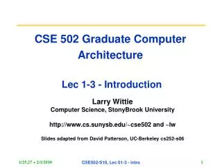
CSE 502 Graduate Computer Architecture Lec 1-3 - Introduction Larry Wittie Computer Science, StonyBrook University http://www.cs.sunysb.edu/~cse502 and ~lw Slides adapted from David Patterson, UC-Berkeley cs252-s06 CSE502-S10, Lec 01-3 - intro
Outline • Computer Science at a Crossroads • Computer Architecture v. Instruction Set Arch. • How would you like your CSE502? • What Computer Architecture brings to table • Quantitative Principles of Design • Technology Performance Trends • Careful, Quantitative Comparisons CSE502-S10, Lec 01-3 - intro
Crossroads: Conventional Wisdom in Comp. Arch • Old Conventional Wisdom: Power is free, Transistors expensive • New Conventional Wisdom: “Power wall” Power expensive, Xtors free (Can put more on chip than can afford to turn on) • Old CW: Can increase Instruction Level Parallelism more via compilers, innovation (Out-of-order, speculation, VLIW, …) • New CW: “ILP wall” law of diminishing returns on more HW for ILP • Old CW: Multiplies are slow, Memory access is fast • New CW: “Memory wall” Memory slow, multiplies fast(200 clock cycles to DRAM memory, 4 clocks for multiply) • Old CW: Uniprocessor performance 2X / 1.5 yrs • New CW: Power Wall + ILP Wall + Memory Wall = Brick Wall • Uniprocessor performance now 2X / 5(?) yrs Sea change in chip design: multiple “cores” (2X processors per chip / ~ 2 years) • Increase on-chip number of simple processors that are power efficient • Simple processor “cores” use less power per useful calculation done CSE502-S10, Lec 01-3 - intro
Crossroads: Uniprocessor Performance From Hennessy and Patterson, Computer Architecture: A Quantitative Approach, 4th edition, October, 2006 • VAX : 25%/year 1978 to 1986 • RISC + x86: 52%/year 1986 to 2002 • RISC + x86: ??%/year 2002 to 2006 CSE502-S10, Lec 01-3 - intro
Sea Change in Chip Design • Intel 4004 (1971): 4-bit processor,2312 transistors, 0.4 MHz, 10 micron PMOS, 11 mm2 chip • RISC II (1983): 32-bit, 5 stage pipeline, 40,760 transistors, 3 MHz, 3 micron NMOS, 60 mm2 chip (6 x 10 mm) • Today (2006) 125 mm2 chip, 0.065 micron CMOS = 2312 RISC II+FPU+Icache+Dcache • RISC II shrinks to ~ 0.02 mm2 at 65 nm • Caches via DRAM or 1 transistor SRAM (www.t-ram.com) ? • Proximity Communication via capacitive coupling at > 1 TB/s ?(Ivan Sutherland @ Sun / Berkeley) • Processor is the new transistor? CSE502-S10, Lec 01-3 - intro
Déjà vu all over again? • Multiprocessors imminent in 1970s, ‘80s, ‘90s, … • “… today’s processors … are nearing an impasse as technologies approach the speed of light..” David Mitchell, The Transputer: The Time Is Now (1989) • Transputer was premature Custom multiprocessors strove to lead uniprocessors Procrastination rewarded: 2X seq. perf. / 1.5 years • “We are dedicating all of our future product development to multicore designs. … This is a sea change in computing” Paul Otellini, President, Intel (2004) • Difference is all microprocessor companies switch to multiprocessors (AMD, Intel, IBM, Sun; all new Apples 2 CPUs) Procrastination penalized: 2X sequential perf. / 5 yrs Biggest programming challenge: going from 1 to 2 CPUs CSE502-S10, Lec 01-3 - intro
Problems with Sea Change • Algorithms, Programming Languages, Compilers, Operating Systems, Architectures, Libraries, … not ready to supply Thread Level Parallelism or Data Level Parallelism for 1000 CPUs / chip, • Architectures not ready for 1000 CPUs / chip • Unlike Instruction Level Parallelism, cannot be solved by just by computer architects and compiler writers alone, but also cannot be solved without participation of computer architects • This edition of CSE 502 (and 4th Edition of textbook Computer Architecture: A Quantitative Approach) explores shift from Instruction Level Parallelism to Thread Level Parallelism / Data Level Parallelism CSE502-S10, Lec 01-3 - intro
Outline • Computer Science at a Crossroads • Computer Architecture v. Instruction Set Arch. • How would you like your CSE502? • What Computer Architecture brings to table • Quantitative Principles of Design • Technology Performance Trends • Careful, Quantitative Comparisons CSE502-S10, Lec 01-3 - intro
Instruction Set Architecture: Critical InterfaceThe computing system as seen by programmers • Properties of a good abstraction • Lasts through many generations (portability) • Used in many different ways (generality) • Provides convenient functionality to higher levels • Permits an efficient implementation at lower levels • What matters today is performance of complete computer systems software instruction set hardware CSE502-S10, Lec 01-3 - intro
Example: MIPS r0 r1 ° ° ° r31 0 Programmable storage 2^32 x bytes 31 x 32-bit GPRs (R0=0) 32 x 32-bit FP regs (paired DP) HI, LO, PC Data types ? Format ? Addressing Modes? PC lo hi • Arithmetic logical • Add, AddU, Sub, SubU, And, Or, Xor, Nor, SLT, SLTU, • AddI, AddIU, SLTI, SLTIU, AndI, OrI, XorI, LUI • SLL, SRL, SRA, SLLV, SRLV, SRAV • Memory Access • LB, LBU, LH, LHU, LW, LWL,LWR • SB, SH, SW, SWL, SWR • Control • J, JAL, JR, JALR • BEq, BNE, BLEZ,BGTZ,BLTZ,BGEZ,BLTZAL,BGEZAL 32-bit instructions on word boundary CSE502-S10, Lec 01-3 - intro
Outline • Computer Science at a Crossroads • Computer Architecture v. Instruction Set Arch. • How would you like your CSE502? • What Computer Architecture brings to table • Quantitative Principles of Design • Technology Performance Trends • Careful, Quantitative Comparisons CSE502-S10, Lec 01-3 - intro
CSE502: Administrivia Instructor: Prof Larry Wittie Office/Lab: 1308 CompSci, lw AT icDOTsunysbDOTedu Office Hours: MW, 3:45 - 5:15 pm, if door open, or appt. T. A.: To Be Determined Class: MW, 2:20 - 3:40 pm 2120 Comp Sci Text: Computer Architecture: A Quantitative Approach, 4th Ed. (Oct, 2006), ISBN 0123704901 or 978-0123704900, $60 Amazon F09 Web page: http://www.cs.sunysb.edu/~cse502/ First reading assignment: Chapter 1 for today, Monday Appendix A (at back of text) for Wednesday CSE502-S10, Lec 01-3 - intro
CSE 502 Course Focus Understanding design techniques, machine structures, technology factors & evaluation methods that will determine the form of computers in 21st Century Parallelism Technology Programming Languages Applications Interface Design (ISA) Computer Architecture: • Organization • Hardware/Software Boundary Compilers Operating Measurement & Evaluation History Systems • Computer architecture is at a crossroads • Institutionalization and renaissance • Power, dependability, multi CPU vs. 1 CPU performance CSE502-S10, Lec 01-3 - intro
Coping with CSE 502 • Undergrads must have taken CSE320 • Grad Students with too varied background? • You will have a difficult time if you have not had an undergrad course using a Hennessy & Patterson text. • Grads without CSE320 equivalent may have to work hard; Review: CSE502 text Appendix A, B, C; the CSE320 home page; and maybe CSE320 text Computer Organization and Design (COD) 3/e • Read chapters 1 to 8 of COD if you never took the prerequisite • If took a class, be sure COD Chapters 2, 6, 7 are very familiar • We will spend 2 week-long lectures on review of Pipelining (App. A) and Memory Hierarchy (App. C), before an in-class quiz to check if everyone is OK. CSE502-S10, Lec 01-3 - intro
Grading • 18% Homeworks (practice for the exams) • 74% Exams: {4% Quiz, 20% Midterm, 50% Final Exam} • 8% (Optional) Research Project (work in pairs) • you need to show initiative • Pick a topic (more on this later) • give oral presentation or poster session • written report like a conference paper • 5 weeks work full-time for 2 people • opportunity to do “research in the small” to help make transition from good undergrad student to research colleague I may add up to 3% to a student’s final score, usually given only to people showing marked improvement during the course. CSE502-S10, Lec 01-3 - intro
Outline • Computer Science at a Crossroads • Computer Architecture v. Instruction Set Arch. • How would you like your CSE502? • What Computer Architecture brings to table • Quantitative Principles of Design • Technology Performance Trends • Careful, Quantitative Comparisons CSE502-S10, Lec 01-3 - intro
What Computer Architecture Brings to Table Quantitative Principles of Design • Take Advantage of Parallelism • Principle of Locality • Focus on the Common Case • Amdahl’s Law • The Processor Performance Equation Culture of anticipating and exploiting advances in technology- technology performance trends Careful, quantitative comparisons • Define, quantify, and summarize relative performance • Define and quantify relative cost • Define and quantify dependability • Define and quantify power Culture of crafting well-defined interfaces that are carefully implemented and thoroughly checked CSE502-S10, Lec 01-3 - intro
1) Taking Advantage of Parallelism • Increasing throughput of server computer via multiple processors or multiple disks • Detailed HW design • Carry lookahead adders uses parallelism to speed up computing sums from linear to logarithmic in number of bits per operand • Multiple memory banks searched in parallel in set-associative caches • Pipelining: overlap instruction execution to reduce the total time to complete an instruction sequence. • Not every instruction depends on immediate predecessor executing instructions completely/partially in parallel possible • Classic 5-stage pipeline: 1) Instruction Fetch (Ifetch), 2) Register Read (Reg), 3) Execute (ALU), 4) Data Memory Access (Dmem), 5) Register Write (Reg) CSE502-S10, Lec 01-3 - intro
Reg Reg Reg Reg Reg Reg Reg Reg ALU Ifetch DMem ALU Ifetch Ifetch Ifetch DMem DMem DMem ALU ALU Time (clock cycles) Cycle 1 Cycle 2 Cycle 3 Cycle 4 Cycle 5 Cycle 6 Cycle 7 I n s t r. O r d e r Pipelined Instruction Execution Is Faster CSE502-S10, Lec 01-3 - intro
Reg Reg Reg Reg Reg Reg Reg Reg Ifetch Ifetch Ifetch Ifetch DMem DMem DMem DMem ALU ALU ALU ALU Limits to Pipelining • Hazards prevent next instruction from executing during its designated clock cycle • Structural hazards: attempt to use the same hardware to do two different things at once • Data hazards: Instruction depends on result of prior instruction still in the pipeline • Control hazards: Caused by delay between the fetching of instructions and decisions about changes in control flow (branches and jumps). Time (clock cycles) I n s t r. O r d e r CSE502-S10, Lec 01-3 - intro
2) The Principle of Locality => Caches ($) • The Principle of Locality: • Programs access a relatively small portion of the address space at any instant of time. • Two Different Types of Locality: • Temporal Locality (Locality in Time): If an item is referenced, it will tend to be referenced again soon (e.g., loops, reuse) • Spatial Locality (Locality in Space): If an item is referenced, items whose addresses are close by tend to be referenced soon (e.g., straight-line code, array access) • For 30 years, HW has relied on locality for memory perf. MEM P $ CSE502-S10, Lec 01-3 - intro
Levels of the Memory Hierarchy Capacity Access Time Cost Staging Xfer Unit Upper Level CPU Registers 100s Bytes 300 – 500 ps (0.3-0.5 ns) Registers prog./compiler 1-8 bytes Instr. Operands Faster L1 Cache L1 and L2 Cache 10s-100s K Bytes ~1 ns - ~10 ns $1000s/ GByte cache cntlr 32-64 bytes Blocks L2 Cache cache cntlr 64-128 bytes Blocks Main Memory G Bytes 80ns- 200ns ~ $100/ GByte Memory OS 4K-8K bytes Pages Disk 10s T Bytes, 10 ms (10,000,000 ns) ~ $0.25 / GByte Disk user/operator Mbytes Files Larger Tape Vault Semi-infinite sec-min ~$1 / GByte Tape Lower Level CSE502-S10, Lec 01-3 - intro
3) Focus on the Common Case“Make Frequent Case Fast and Rest Right” • Common sense guides computer design • Since its engineering, common sense is valuable • In making a design trade-off, favor the frequent case over the infrequent case • E.g., Instruction fetch and decode unit used more frequently than multiplier, so optimize it first • E.g., If database server has 50 disks / processor, storage dependability dominates system dependability, so optimize it 1st • Frequent case is often simpler and can be done faster than the infrequent case • E.g., overflow is rare when adding 2 numbers, so improve performance by optimizing more common case of no overflow • May slow down overflow, but overall performance improved by optimizing for the normal case • What is frequent case and how much performance improved by making case faster => Amdahl’s Law CSE502-S10, Lec 01-3 - intro
Example: An I/O bound server gets a new CPU that is 10X faster, but 60% of server time is spent waiting for I/O. 4) Amdahl’s Law - Partial Enhancement Limits Best to ever achieve: A 10X faster CPU allures, but the server is only 1.6X faster. CSE502-S10, Lec 01-3 - intro
CPU time = Seconds = Instructions x Cycles x Seconds Program Program Instruction Cycle CPI 5) Processor performance equation Inst count CPU time = Inst Count x CPI x Clock Cycle Program X Compiler X (X) Inst. Set. X X Organization X X Technology X Cycle time CSE502-S10, Lec 01-3 - intro
What Determines a Clock Cycle? • At transition edge(s) of each clock pulse, state devices sample and save their present input signals • Past: 1 cycle = time for signals to pass 10 levels of gates • Today: determined by numerous time-of-flight issues + gate delays • clock propagation, wire lengths, drivers Latch or register combinational logic CSE502-S10, Lec 01-3 - intro
What Computer Architecture brings to Table Quantitative Principles of Design • Take Advantage of Parallelism • Principle of Locality • Focus on the Common Case • Amdahl’s Law • The Processor Performance Equation Culture of anticipating and exploiting advances in technology- technology performance trends Careful, quantitative comparisons • Define, quantify, and summarize relative performance • Define and quantify relative cost • Define and quantify dependability • Define and quantify power Culture of well-defined interfaces that are carefully implemented and thoroughly checked CSE502-S10, Lec 01-3 - intro
Moore’s Law: 2X transistors / “year [or 2]” “Cramming More Components onto Integrated Circuits” • Gordon Moore, Electronics, 1965 # on transistors / cost-effective integrated circuit double every N months (12 ≤ N ≤ 24) CSE502-S10, Lec 01-3 - intro
Tracking Technology Performance Trends • Drill down into 4 technologies: • Disks, • Memory, • Network, • Processors • Compare ~1980 Archaic (Nostalgic) vs. ~2000 Modern (Newfangled) • Performance Milestones in each technology • Compare for Bandwidth vs. Latency improvements in performance over time • Bandwidth: number of events per unit time • E.g., M bits / second over network, M bytes / second from disk • Latency: elapsed time for a single event • E.g., one-way network delay in microseconds, average disk access time in milliseconds CSE502-S10, Lec 01-3 - intro
Seagate 373453, 2003 15000 RPM (4X) 73.4 GBytes (2500X) Tracks/Inch: 64,000 (80X) Bits/Inch: 533,000 (60X) Four 2.5” platters (in 3.5” form factor) Bandwidth:86 MBytes/sec (140X) Latency: 5.7 ms (8X) Cache: 8 MBytes CDC Wren I, 1983 3600 RPM 0.03 GBytes capacity Tracks/Inch: 800 Bits/Inch: 9,550 Three 5.25” platters Bandwidth: 0.6 MBytes/sec Latency: 48.3 ms Cache: none Disks: Archaic(Nostalgic) v. Modern(Newfangled) CSE502-S10, Lec 01-3 - intro
Performance Milestones Disk: 3600, 5400, 7200, 10000, 15000 RPM (8x, 143x) Latency Lags Bandwidth (for last ~20 years) (Latency = simple operation w/o contention, BW = best-case) CSE502-S10, Lec 01-3 - intro
1980 DRAM(asynchronous) 0.06 Mbits/chip 64,000 xtors, 35 mm2 16-bit data bus per module, 16 pins/chip 13 Mbytes/sec Latency: 225 ns (no block transfer) 2000Double Data Rate Synchr. (clocked) DRAM 256.00 Mbits/chip (4000X) 256,000,000 xtors, 204 mm2 64-bit data bus per DIMM, 66 pins/chip (4X) 1600 Mbytes/sec (120X) Latency: 52 ns (4X) Block transfers (page mode) Memory: Archaic (Nostalgic) v. Modern (Newfangled) CSE502-S10, Lec 01-3 - intro
Performance Milestones Memory Module: 16bit plain DRAM, Page Mode DRAM, 32b, 64b, SDRAM, DDR SDRAM (4x,120x) Disk:3600, 5400, 7200, 10000, 15000 RPM (8x, 143x) Latency Lags Bandwidth (for last ~20 years) (Latency = simple operation w/o contention, BW = best-case) CSE502-S10, Lec 01-3 - intro
Ethernet 802.3 Year of Standard: 1978 10 Mbits/s link speed Latency: 3000 msec Shared media Coaxial cable "Cat 5" is 4 twisted pairs in bundle Twisted Pair: Copper, 1mm thick, twisted to avoid antenna effect LANs: Archaic (Nostalgic) v. Modern (Newfangled) • Ethernet 802.3ae • Year of Standard: 2003 • 10,000 Mbits/s (1000X)link speed • Latency: 190 msec (15X) • Switched media • Category 5 copper wire Coaxial Cable: Plastic Covering Braided outer conductor Insulator Copper core CSE502-S10, Lec 01-3 - intro
Performance Milestones Ethernet: 10Mb, 100Mb, 1000Mb, 10000 Mb/s (16x,1000x) Memory Module:16bit plain DRAM, Page Mode DRAM, 32b, 64b, SDRAM, DDR SDRAM (4x,120x) Disk:3600, 5400, 7200, 10000, 15000 RPM (8x, 143x) Latency Lags Bandwidth (for last ~20 years) (Latency = simple operation w/o contention, BW = best-case) CSE502-S10, Lec 01-3 - intro
1982 Intel 80286 12.5 MHz 2 MIPS (peak) Latency 320 ns 134,000 xtors, 47 mm2 16-bit data bus, 68 pins Microcode interpreter, separate FPU chip (no caches) 2001 Intel Pentium 4 1500MHz = 1.5 GHz (120X) 4500 MIPS (peak) (2250X) Latency 15 ns (20X) 42,000,000 xtors, 217 mm2 64-bit data bus, 423 pins 3-way superscalar,Dynamic translate to RISC, Superpipelined (22 stage),Out-of-Order execution On-chip 8KB Data caches, 96KB Instr. Trace cache, 256KB L2 cache CPUs: Archaic (Nostalgic) v. Modern (Newfangled) CSE502-S10, Lec 01-3 - intro
Performance Milestones Processor: ‘286, ‘386, ‘486, Pentium, Pentium Pro, Pentium 4 (21x,2250x) Ethernet: 10Mb, 100Mb, 1000Mb, 10000 Mb/s (16x,1000x) Memory Module: 16bit plain DRAM, Page Mode DRAM, 32b, 64b, SDRAM, DDR SDRAM (4x,120x) Disk : 3600, 5400, 7200, 10000, 15000 RPM (8x, 143x) CPU high, Memory low(“Memory Wall”) Δ.Latency Lags Δ.Bandwidth (for last 20 yrs) (Latency = simple operation w/o contention, BW = best-case) CSE502-S10, Lec 01-3 - intro
6 Reasons LatencyLags Bandwidth 1. Moore’s Law helps BW more than latency • Faster transistors, more transistors, more pins help Bandwidth (cf.,MicroProcessing Unit, Dynamic RAM) • MPU Transistors: 0.130 vs. 42 M xtors (300X) • DRAM Transistors: 0.064 vs. 256 M xtors (4000X) • MPU Pins: 68 vs. 423 pins (6X) • DRAM Pins: 16 vs. 66 pins (4X) • Smaller, faster transistors but communicating over (relatively) longer lines: limits latency • Feature size: 1.5 to 3 vs. 0.18 micron (8X,17X) • MPU Die Size: 35 vs. 204 mm2 (ratio sqrt 2X) • DRAM Die Size: 47 vs. 217 mm2 (ratio sqrt 2X) CSE502-S10, Lec 01-3 - intro
6 Reasons LatencyLags Bandwidth (cont’d) 2. Distance limits latency • Size of DRAM block long bit and word lines most of DRAM access time • Speed of light and computers on network • 1. & 2. explains linear latency vs. square BW? 3. Bandwidth easier to sell (“bigger=better”) • E.g., 10 Gbits/s Ethernet (“10 Gig”) vs. 10 msec latency Ethernet • 4400 MB/s DIMM (“PC4400”) vs. 50 ns latency • Even if it is just marketing, customers are now trained • Since bandwidth sells, more resources thrown at bandwidth, which further tips the balance CSE502-S10, Lec 01-3 - intro
6 Reasons LatencyLags Bandwidth (cont’d) 4. Latency helps BW, but not vice versa • Spinning disk faster improves both bandwidth and rotational latency • 3600 RPM 15000 RPM = 4.2X • Average rotational latency: 8.3 ms 2.0 ms • Things being equal, also helps BW by 4.2X • Lower DRAM latency More access/second (higher bandwidth) • Higher linear density helps disk BW (and capacity), but not disk Latency • 9,550 BPI 533,000 BPI 60X in BW CSE502-S10, Lec 01-3 - intro
6 Reasons LatencyLags Bandwidth (cont’d) 5. Bandwidth hurts latency • Queues help Bandwidth, hurt Latency (Queuing Theory) • Adding chips to widen a memory module increases Bandwidth but higher fan-out on address lines may increase Latency 6. Operating System overhead hurts Latency more than Bandwidth • Long messages amortize overhead; overhead bigger part of short messages It takes longer to create and to send a long message, which is needed instead of a short message to lessen average cost per data byte of fixed size message overhead. “Bandwidth problems can be solved with $$, latency problems need prayer (to make light go faster).” CSE502-S10, Lec 01-3 - intro
Summary of Technology Trends • For disk, LAN, memory, and microprocessor, bandwidth improves by more than the square of latency improvement • In the time that bandwidth doubles, latency improves by no more than 1.2X to 1.4X • Lag of gains for latency vs bandwidth probably even larger in real systems, as bandwidth gains multiplied by replicated components • Multiple processors in a cluster or even on a chip • Multiple disks in a disk array • Multiple memory modules in a large memory • Simultaneous communication in switched local area networks (LANs) • HW and SW developers should innovate assuming Latency Lags Bandwidth • If everything improves at the same rate, then nothing really changes • When rates vary, good designs require real innovation CSE502-S10, Lec 01-3 - intro
Outline • Computer Science at a Crossroads • Computer Architecture v. Instruction Set Arch. • How would you like your CSE502? • Technology Trends: Culture of tracking, anticipating and exploiting advances in technology • Careful, quantitative comparisons: • Define and quantify power • Define and quantify dependability • Define, quantify, and summarize relative performance CSE502-S10, Lec 01-3 - intro
Define and quantify power ( 1 / 2) • For CMOS chips, traditional dominant energy use has been in switching transistors, called dynamic power • For mobile devices, energy is a better metric • For a fixed task, slowing clock rate (the switching frequency) reduces power, but not energy • Capacitive load is function of number of transistors connected to output and the technology, which determines the capacitance of wires and transistors • Dropping voltage helps both, so ICs went from 5V to 1V • To save energy & dynamic power, most CPUs now turn off clock of inactive modules (e.g. Fltg. Pt. Arith. Unit) • If a 15% voltage reduction causes a 15% reduction in frequency, what is the impact on dynamic power? • New power/old = 0.852 x 0.85 = 0.853 = 0.614 “39% reduction” • {volt2 x freq} CSE502-S10, Lec 01-3 - intro
Define and quantify power (2 / 2) • Because leakage current flows even when a transistor is off, now static power important too • Leakage current increases in processors with smaller transistor sizes • Increasing the number of transistors increases power even if they are turned off • In 2006, the goal for leakage is 25% of total power consumption; high performance designs allow 40% • Very low power systems even gate voltage to inactive modules to reduce losses because of leakage currents CSE502-S10, Lec 01-3 - intro
Outline • Computer Science at a Crossroads • Computer Architecture v. Instruction Set Arch. • How would you like your CSE502? • Technology Trends: Culture of tracking, anticipating and exploiting advances in technology • Careful, quantitative comparisons: • Define and quantify power • Define and quantify dependability • Define, quantify, and summarize relative performance CSE502-S10, Lec 01-3 - intro
Define and quantify dependability (1/3) • How to decide when a system is operating properly? • Infrastructure providers now offer Service Level Agreements (SLA) which are guarantees how dependable their networking or power service will be • Systems alternate between two states of service: • Service accomplishment (working), where the service is delivered as specified in SLA • Service interruption (not working), where the delivered service is different from the SLA • Failure = transition from state 1 (working) to state 2 • Restoration = transition from state 2 (not) to state 1 CSE502-S10, Lec 01-3 - intro
Define and quantity dependability (2/3) • Module reliability = measure of continuous service accomplishment (or time to failure). • Mean Time To Failure (MTTF) measures Reliability • Failures In Time (FIT) = 1/MTTF, the failure rate • Usually reported as failures per billion hours of operation • Mean Time To Repair (MTTR) measures Service Interruption • Mean Time Between Failures (MTBF) = MTTF+MTTR • Module availability measures service as alternate between the two states of accomplishment and interruption (number between 0 and 1, e.g. 0.9) • Module availability = MTTF / ( MTTF + MTTR) CSE502-S10, Lec 01-3 - intro
Example calculating reliability • If modules have exponentially distributed lifetimes (the age of a module does not affect its probability of failure), the overall failure rate (FIT) is the sum of failure rates of the modules • Calculate FIT (rate) and MTTF (1/rate) for 10 disks (1M hour MTTF per disk), 1 disk controller (0.5M hour MTTF), and 1 power supply (0.2M hour MTTF): { x 109 } CSE502-S10, Lec 01-3 - intro
Outline • Computer Science at a Crossroads • Computer Architecture v. Instruction Set Arch. • How would you like your CSE502? • Technology Trends: Culture of tracking, anticipating and exploiting advances in technology • Careful, quantitative comparisons: • Define and quantify power • Define and quantify dependability • Define, quantify, and summarize relative performance CSE502-S10, Lec 01-3 - intro