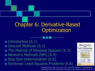
Chapter 6: Derivative-Based Optimization
Chapter 6: Derivative-Based Optimization. Introduction (6.1) Descent Methods (6.2) The Method of Steepest Descent (6.3) Newton’s Methods (NM) (6.4) Step Size Determination (6.5) Nonlinear Least-Squares Problems (6.8).

Chapter 6: Derivative-Based Optimization
E N D
Presentation Transcript
Chapter 6: Derivative-Based Optimization Introduction (6.1) Descent Methods (6.2) The Method of Steepest Descent (6.3) Newton’s Methods (NM) (6.4) Step Size Determination (6.5) Nonlinear Least-Squares Problems (6.8) Jyh-Shing Roger Jang et al., Neuro-Fuzzy and Soft Computing: A Computational Approach to Learning and Machine Intelligence, First Edition, Prentice Hall, 1997
Introduction (6.1) • Goal: Solving minimization nonlinear problems through derivative information • We cover: • Gradient based optimization techniques • Steepest descent methods • Newton Methods • Conjugate gradient methods • Nonlinear least-squares problems • They are used in: • Optimization of nonlinear neuro-fuzzy models • Neural network learning • Regression analysis in nonlinear models Dr. Djamel Bouchaffra
Descent methods (6.2) • Goal:Determine a point such that f(1, 2, …, n) is minimum on • We are looking for a local & not necessarily a global minimum • Let f(1, 2, …, n) = E(1, 2, …, n), the search of this minimum is performed through a certain direction d starting from an initial value = 0 (iterative scheme!) Dr. Djamel Bouchaffra
Descent Methods (6.2) (cont.) next = now + d ( > 0 is a step size regulating the search in the direction d) k +1 = k + kdk (k = 1, 2, …) The series should converge to a local minimum • We first need to determine the next direction d & then compute the step size • kdk is called the k-th step, whereas k is the k-th step size • We should have E(next) = E(now + d) < E(now) • The principal differences between various descent algorithms lie in the first procedure for determining successive directions Dr. Djamel Bouchaffra
Descent Methods (6.2) (cont.) • Once d is determined, is computed as: • Gradient-based methods • Definition:The gradient of a differentiable function E: IRn IR at is the vector of first derivatives of E, denoted as g. That is: Dr. Djamel Bouchaffra
Descent Methods (6.2) (cont.) • Based on a given gradient, downhill directions adhere to the following condition for feasible descent directions: Where is the angle between g and d and (now) is the angle between gnow and d at point now Dr. Djamel Bouchaffra
Descent models (6.2) (cont.) The previous equation is justified by Taylor series expansion: E(now + d) = E(now) + gTd + 0(2) Dr. Djamel Bouchaffra
Descent Methods (6.2) (cont.) • A class of gradient-based descent methods has the following form in which feasible descent directions can be found by gradient deflection • Gradient deflection consists of multiplying the gradient g by a positive definite matrix (pdm) G d = - Gg gTd = - gTGg < 0 (feasible descent direction) • The gradient-based method is described therefore by: next = now - Gg ( > 0, G pdm) (*) Dr. Djamel Bouchaffra
Descent Methods (6.2) (cont.) • Theoretically, we wish to determine a value next such as: but this is difficult to solve!! • But practically, we stop the algorithm if: • The objective function value is sufficiently small • The length of the gradient vector g is smaller than a threshold • The computation time is exceeded (Necessary condition but not sufficient!) Dr. Djamel Bouchaffra
The method of Steepest Descent (6.3) • Despite its slow convergence, this method is the most frequently used nonlinear optimization technique due to its simplicity • If G = Id (identity matrix) then equation (*) expresses the steepest descent scheme: next = now - g • If Cos = -1 (meaning that d points to the same direction of vector – g ) then the objective function E can be decreased locally by the biggest amount at point now Dr. Djamel Bouchaffra
The method of Steepest Descent (6.3) (cont.) • Therefore, the negative gradient direction (-g) points to the locally steepest downhill direction • This direction may not be a shortcut to reach the minimum point * • However, if the steepest descent uses the line minimization technique (min ()) then ’() = 0 gnext is orthogonal to the current gradient vector gnow(see figure 6.2; pt X) (Necessary Condition for ) Dr. Djamel Bouchaffra
The method of Steepest Descent (6.3) (cont.) • If the contours of the objective function E form hyperspheres (or circles in a 2 dimensional space), the steepest descent methods leads to the minimum in a single step. Otherwise the method does not lead to the minimum point Dr. Djamel Bouchaffra
Newton’s Methods (NM) (6.4) • Classical NM • Principle:The descent direction d is determined by using the second derivatives of the objective function E if available • If the starting position now is sufficient close to a local minimum, the objective function E can be approximated by a quadratic form: Dr. Djamel Bouchaffra
Newton’s Methods (NM) (6.4) (cont.) • Since the equation defines a quadratic function E() in the now neighborhood its minimum can be determined by differenting & setting to 0. Which gives: 0 = g + H( - now) Equivalent to: = now – H-1g • It is a gradient-based method for = 1 and G = H-1 Dr. Djamel Bouchaffra
Newton’s Methods (NM) (6.4) (cont.) • Only when the minimum point of the approximated quadratic function is chosen as the next point next, we have the so-called NM or the Newton-Raphson method = now – H-1g • If H is positive definite and E() is quadratic then the NM directly reaches a local minimum in the single Newton step (single – H-1g) • If E() is not quadratic, then the minimum may nor be reached in a single step & NM should be iteratively repeated Dr. Djamel Bouchaffra
Step Size Determination (6.5) • Formula of a class of gradient-based descent methods: next = now + d = now - Gg • This formula entails effectively determining the step size • ’() = 0 with () = E( now+ d) is often impossible to solve Dr. Djamel Bouchaffra
Step Size Determination (6.5) (cont.) • Initial Bracketing • We assume that the search area (or specified interval) contains a single relative minimum: E is unimodal over the closed interval • Determining the initial interval in which a relative minimum must lie is of critical importance • A scheme, by function evaluation for finding three points to satisfy: E(k-1) > E(k) < E(k+1); k-1 < k < k+1 • A scheme, by taking the first derivative, for finding two points to satisfy: • E’(k) < 0, E’(k+1) > 0, k < k+1 Dr. Djamel Bouchaffra
Algorithm for scheme 1: An initial bracketing for searching three points 1, 2 and 3 1) Given a starting point 0 and h IR, let 1 be 0 +h. Evaluate E(1)if E(0) E(1), i 1(i.e., go downhill)go to (2)otherwise h -h (i.e., set backward direction) E (-1) E(1) 1 0 + h i 0 go to(3) 2) Set the next point by; h 2h, i+1 i + h 3) Evaluate E(i+1)if E(i) E(i+1); i i + 1 (i.e., still go downhill) go to (2) Otherwise, Arrange i-1, i and i+1 in the decreasing order Then, we obtain the three points: (1,2,3) Stop. Dr. Djamel Bouchaffra
Step Size Determination (6.5) (cont.) • Line searches • The process of determining * that minimizes a one-dimensional function () is achieved by searching on the line for the minimum • Line search algorithms usually include two components: sectioning (or bracketing), and polynomial interpolation • Newton’s methodWhen (k), ’(k), and ’’(k) are available, the classical Newton method (defined by ) can be applied to solving the equation ’(k) = 0: Dr. Djamel Bouchaffra
Step Size Determination (6.5) (cont.) • Secant method If we use both k and k-1 to approximate the second derivative in equation (*), and if the first derivatives alone are available then we have an estimated k+1 defined as: this method is called the secant method. Both the Newton’s and the secant method are illustrated in the following figure. Dr. Djamel Bouchaffra
Newton’s method and secant method to determinethe step size Dr. Djamel Bouchaffra
Step Size Determination (6.5) (cont.) • Sectioning methods • It starts with an interval [a1, b1] in which the minimum must lie, and then reduces the length of the interval at each iteration by evaluating the value of at a certain number of points • The two endpoints a1 and b1 can be found by the initial bracketing described previously • The bisection method is one of the simplest sectioning method for solving ’(*) = 0, if first derivatives are available! Dr. Djamel Bouchaffra
Let ’() = () then the algorithm is: Algorithm [bisection method] (1) Given IR+ and an initial interval with 2 endpoints a1 and a2 such that: a1 < a2 and (a1)(a2) < 0 then set: left a1 right a2 (2) Compute the midpoint mid; mid (right + left) / 2 if (right) (mid) < 0, left mid Otherwise right mid (3) Check if |left -right| < . If it is true then terminate the algorithm, otherwise go to (2) Dr. Djamel Bouchaffra
Step Size Determination (6.5) (cont.) • Golden section search method This method does not require to be differentiable. Given an initial interval [a1,b1] that contains , the next trial points (sk,tk) within the interval are determined by using the golden section ratio : Dr. Djamel Bouchaffra
Step Size Determination (6.5) (cont.) This procedure guarantees the following: ak < sk < tk < bk The algorithm generates a sequence of two endpoints ak and bk, according to: If (sk) > (tk), ak+1 = sk, bk+1 = bk Otherwise ak+1 = ak, bk+1 = tk The minimum point is bracketed to an interval just 2/3 times the length of the preceding interval Dr. Djamel Bouchaffra
Golden section search to determine the step length Dr. Djamel Bouchaffra
Step Size Determination (6.5) (cont.) • Line searches (cont.) • Polynomial interpolation • This method is based on curve-fitting procedures • A quadratic interpolation is the method that is very often used in practice • It constructs a smooth quadratic curve q that passes through three points (1, 1), (2, 2) and (3, 3): where i = (i), i = 1, 2, 3 Dr. Djamel Bouchaffra
Step Size Determination (6.5) (cont.) • Polynomial interpolation (cont.) • Condition for obtaining a unique minimum point is: q’() = 0, therefore the next point next is: Dr. Djamel Bouchaffra
Quadratic Interpolation Dr. Djamel Bouchaffra
Step Size Determination (6.5) (cont.) • Termination rules • Line search methods do not provide the exact minimum point of the function • We need a termination rule that accelerate the entire minimization process without affecting too much precision Dr. Djamel Bouchaffra
Step Size Determination (6.5) (cont.) • Termination rules (cont.) • The Goldstein Test • This method is based on two definitions: • A value of is not too large if with a given (0 < < ½), () (0) + ’(0) • A value of is considered to be not too small if: () > (0) + (1 - ) ’() Dr. Djamel Bouchaffra
Step Size Determination (6.5) (cont.) • Goldstein test (cont.) • From the two precedent inequalities, we obtain: (1 - ) ’(0) () - (0) = E(next) – E(now) ’(0) which can be written as: where ’(0) = gTd < 0 (Taylor series) (Condition for !) Dr. Djamel Bouchaffra
Goldstein Test Dr. Djamel Bouchaffra
Nonlinear Least-Squares Problems (6.8) • Goal:Optimize a model by minimizing a squared error measure between desired outputs & the model’s output y = f(x, ) Given a set of m training data pairs (xp; tp), (p = 1, …, m), we can write: Dr. Djamel Bouchaffra
Nonlinear Least-Squares Problems (6.8) (cont.) • The gradient is expressed as: where J is the Jacobian matrix of r. Since rp() = tp – f(xp, ), this implies that the pth row of J is: Dr. Djamel Bouchaffra
Nonlinear Least-Squares Problems (6.8) (cont.) • Gauss-Newton Method • Known also as the linearization method • Use Taylor series expansion to obtain a linear model that approximates the original nonlinear model • Use linear least-squares optimization of chapter 5 to obtain the model parameters Dr. Djamel Bouchaffra
Nonlinear Least-Squares Problems (6.8) (cont.) • Gauss-Newton Method (cont.) • The parameters T = (1, 2, …, n,…) will be computed iterativelly • Taylor expansion of y = f(x, ) around = now Dr. Djamel Bouchaffra
Nonlinear Least-Squares Problems (6.8) (cont.) • Gauss-Newton Method (cont.) • y – f(x, now) is linear with respect to i - i,now since the partial derivatives are constant where S = - now Dr. Djamel Bouchaffra
Nonlinear Least-Squares Problems (6.8) (cont.) • Gauss-Newton Method (cont.) • The next point next is obtained by: • Therefore, the following Gauss-Newton formula is expressed as: next = now – (JTJ)-1 JTr = now – ½ (JTJ)-1g (since g = 2JTr) Dr. Djamel Bouchaffra