Tensor Product Volumes and Multivariate Methods
Tensor Product Volumes and Multivariate Methods. CAGD Presentation by Eric Yudin June 27, 2012. Multivariate Methods: Outline. Introduction and Motivation Theory Practical Aspects Application: Free-form Deformation (FFD). Introduction and Motivation.

Tensor Product Volumes and Multivariate Methods
E N D
Presentation Transcript
Tensor Product Volumes and Multivariate Methods CAGD Presentation by Eric Yudin June 27, 2012
Multivariate Methods: Outline • Introduction and Motivation • Theory • Practical Aspects • Application: Free-form Deformation (FFD)
Introduction and Motivation • Until now we have discussed curves ( ) and surfaces ( ) in space. • Now we consider higher dimensional – so-called “multivariate” objects in
Introduction and Motivation Examples • Scalar or vector-valued physical fields (temperature, pressure, etc. on a volume or some other higher-dimensional object)
Introduction and Motivation Examples • Spatial or temporal variation of a surface (or higher dimensions)
Introduction and Motivation Examples • Freeform Deformation
Multivariate Methods: Outline • Introduction and Motivation • Theory • Practical Aspects • Application: Free-form Deformation (FFD)
Theory – General Form Definition (21.1): The tensor product B-spline function in three variables is called a trivariate B-spline function and has the form It has variable ui, degree ki, and knot vector ti in the ith dimension
Theory – General Form Definition (21.1) (cont.): Generalization to arbitrary dimension q: • Determining the vector of polynomial degree in each of the q dimensions, n, (?), forming q knot vectors ti, i=1, …, q • Let m=(u1, u2, …, uq) • Let i= (i1, i2, …, iq), where each ij, j=1, …, q • q-variate tensor product function: Of degrees k1, k2, …, kq in each variable
Theory – General Form • is a multivariate function from to given that • If d > 1, then T is a vector (parametric function)
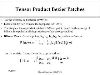
Theory – General Form Definition for Béziertrivariates : A Tensor-Product Bézier volume of degree (l,m,n) is defined to be where and are the Bernstein polynomials of degree , index . Béziertrivariates can similarly be generalized to an arbitrary-dimensional multivariate.
Theory From here on, unless otherwise specified, we will concern ourselves only with Béziertrivariates and multivariates.
Theory – Operations & Properties • Convex Hull Property: All points defined by the Tensor Product Volume lie inside the convex hull of the set of points . • Parametric Surfaces: Holding one dimension of a Tensor Product BézierVolume constant creates a Béziersurface patch – specifically, an isoparametric surface patch. • Parametric Lines: Holding two dimensions of a Tensor Product BézierVolume constant creates a Bézier curve – again, an isoparametric curve.
Theory – Operations and Properties • Boundary surfaces: The boundary surfaces of a TPB volume are TPB surfaces. Their Bézier nets are the boundary nets of the Bézier grid. • Boundary curves: The boundary curves of a TPB volume are Bézier curve segments. Their Bézier polygons are given by the edge polygons of the Bézier grid. • Vertices: The vertices of a TPB volume coincide with the vertices of its Bézier grid.
Theory – Operations and Properties Derivatives: The partial derivatives of order of a Tensor Product Bézier volume of degree ( at the point u = is given by Where the forward difference operator is: and
Theory – Operations and Properties Degree Raising: To raise a Tensor Product Bezier volume of degree to degree , then the new points This works similarly for the other dimensions as well.
Theory – Operations and Properties Degree Reduction: To lower a Tensor Product Bezier volume of degree to one of degree , we need: Then the new points are given recursively by: Each iteration reduces the degree of the dimension of interest by 1. This works similarly for the other dimensions as well.
Theory – Terminology Isosurfaces: In constrast to isoparametric surfaces, an isosurface, or constant set is generated when the Tensor Product Bezier Volume function is set to a constant: Data-wise, this might represent all of the locations in space having equal temperature, pressure, etc. An isosurface is an implicit surface.
Theory – constructors Extruded Volume & Ruled Volume
Theory – constructors Extruded Volume: A surface crossed with a line. Let and be a parametric spline surface and a unit vector, respectively. Then represents the volume extruded by the surface as it is moved in direction It is linear in .
Theory – constructors Ruled Volume: A linear interpolation between two surfaces. Let and be two parametric spline surfaces in the same space (i.e., with the same order and knot sequence). Then the trivariate constructs a ruled volume between and .
Multivariate Methods: Outline • Introduction and Motivation • Theory • Practical Considerations • Application: Free-form Deformation (FFD)
Application: Free-form Deformation Introduction & Motivation: • Embed curves, surfaces and volumes in the parameter domain of a free-form volume • Then modify that volume to warp the inner objects on a ‘global’ scale • [DEMO]
Application: Free-form Deformation Process (Bézier construction): • Obtain/construct control point structure (the FFD) • Transform coordinates to FFD domain • Embed object into the FFD equation From the paper: Sederberg, Parry: “Free-form Deormation of Solid Geometric Models.” ACM 20 (1986) 151-160.
Application: Free-form Deformation Obtain/construct control point structure (the FFD): A common example is a lattice of points P such that: Where • is the origin of the FFD space • S, T, U are the axes of the FFD space • l, m, n are the degrees of each Bézier dimension • i, j, k are the indices of points in each dimension • Edges mapped into Bézier curves
Application: Free-form Deformation Transform coordinates to FFD domain: Any world point has coordinates in this system such that: So X in FFD space is given by the coordinates:
Application: Free-form Deformation Embed object into the FFD equation: The deformed position of the coordinates are given by:
Application: Free-form Deformation Embed object into the FFD equation: If the coordinates of our object are given by: and then we simply embed via:
Application: Free-form Deformation Volume Change: If the FFD is given by and the volume of any differential element is , then its volume after the deformation is where J is the Jacobian, defined by:
Application: Free-form Deformation Volume Change Results: • If we can obtain a bound on over the deformation region, then we have a bound on the volume change. • There exists a family of FFDs for which , i.e., the FFD preserves volume.
Application: Free-form Deformation Examples • Surfaces (solid modeling) • Text (one dimension lower): Text Sculpt [DEMO]
Multivariate Methods: Outline • Introduction and Motivation • Theory • Practical Considerations • Application: Free-form Deformation (FFD)
Practical Aspects – Evaluation • Tensor Product Volumes are composed of Tensor Product Surfaces, which in turn are composed of Bezier curves. • Everything is separable, so each component can be handled independently
Practical Aspects – Visualization Marching Cubes Algorithm • Split space up into cubes • For each cube, figure out which points are inside the iso-surface • 28=256 combinations, which map to 16 unique cases via rotations and symmetries • Each case has a configuration of triangles (for the linear case) to draw within the current cube
Practical Aspects – Visualization Marching Cubes Algorithm: 2D case With ambiguity in cases 5 and 10
Practical Aspects – Visualization Marching Cubes Algorithm: 3D case. Generalizable by 15 families via rotations and symmetries.