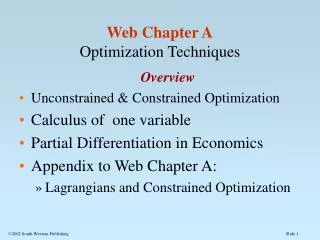
Optimization Techniques Lecture 2 (Appendix C)
Optimization Techniques Lecture 2 (Appendix C). Optimization Techniques. . Optimization is: a process by which the maximum or minimum values of decision variables are determined. Examples Finding the profit maximizing PC sales units at Dell, or at COMPAQ, or at IBM.

Optimization Techniques Lecture 2 (Appendix C)
E N D
Presentation Transcript
Optimization Techniques • . Optimization is: • a process by which the maximum or minimum values of decision variables are determined. • Examples • Finding the profit maximizing PC sales units at Dell, or at COMPAQ, or at IBM. • Finding the cost minimizing units of product line at Nissan(Trucks, Sentra, Altima)
2. Economic relationships can be expressed in the form of tables,graphs, or equations.
TR • 0 0 • 90 • 160 • 210 • 240 • 250 • 240 2a. Table 2b. graph QTR TR Q
Economic Relationships 2c. Equation TR=100Q-10Q2
3. An optimal sales value for profit maximization can be obtained by a total, or marginal approach. Total Approach: Profit is maximized when TR-TC is maximum at Q* Illustrate graphically Marginal Approach:Profit is maximized when MR=MC or MR-MC=O at Q*
Total Approach TR TC TC Profit is max at Q* because TR-TC is Max TR Q Q* maximizes profit
Marginal Approach MR MC MC MR Q Q*
Marginal analysis- a technique which postulates that an activity should be carried out until the marginal benefit (MB) equals the marginal cost (MC). • . When the total value reaches maximum, the marginal (additional)value will be zero(See page C-12 in the book) Given: π=100Q-10Q2 Illustrate
.A derivative is simply a mathematical procedure for obtaining the marginal value (or slope)of a parent function at a point as the change in the explanatory variable approaches 0. Given: y= f(x) as a parent function then, dy/dx=lim(ΔY/ΔX):marginal value as ΔX0 = (a slope at a point). Example: If y=f(x-4), what is the limit of the function y as x5? 1 = 5-4.
.A review of the Rules of Differentiation Rule 1:Constant: The derivative of a constant is always zero. Given: y= f(x)= 2000 dy/dx= 0 y=$2000 TFC= f(Q)= $2000 dTFC/dQ=0 Y Y=2000 X
Rule 2: Power Function: The first derivative of a power function such as y=aXb where a & b are constants, is equal to the exponent b multiplied by a times the variable x raised to b-1 power Given y=axb dy/dx=b.axb-1 e.g. y=2x3 dy/dx=3.2x3-1=6x2 (We do it in our heads!)
Rule 3: Sums and Differences The derivative of a sum (difference) is equal to the derivative of the individual terms. Given: y=u+v where u=f(x) and v=g(x) or y=u-v, then dy/dx=du/dx + dv/dx or dy/dx=du/dx-dv/dx y=9x2+2x+3 y=9x2-2x-3 dy/dx =18x+2 or dy/dx=18x-2
Rule 4: Products Rule The derivative of the product of two expressions is equal to the sum of the first term multiplied by the derivative of the second plus the second term times the derivative of the first.
Rule 4: Products Rule Given:y = U.V and U & V = f(x) dy/dx= U dv/dx +V du/dx y = 3x2(3-x);Let u = 3x2; v = 3-x Then dy/dx =3x2(-1) + (3-x)(6x) =-3x2+18x-6x2= 18x - 9x2
Rule 5: Quotient Rule: The derivative of a quotient of two expressions is equal to the denominator multiplied by the derivative of the numerator minus the numerator times the derivative of the denominator all divided by the square of the denominator.
Rule 5: Quotient Rule Given: y=u/v where u and v= f(x) dy/dx = V.du/dx – U.dv/dx V2 If Y= (2x-3)/6x2, then dy/dx = 6x2(2) - (2x-3) 12x (6x2)2 = [-12x2 +36x]/36x4]
Rule 6: A Function of a Function (Chain Rule):the derivative of such a function is found as follows: Given: y=f(u) where u=g x) Then dy/dx=(dy/du)(du/dx) e.g. Y= 2U-U2; and U =2x3 Then dy/dx= (2-2U)6x2, or after substituting U =2x3 =[2-2(2x3)]6x2 =12x2-24x5
Rule 7: Logarithmic function: Given y = lnx dy/dx= dlnx/dx=1/x
. Use of a derivative in the optimization process. Step 1: Helps to Identify: the maximum or minimum values of decision variables (Q, Ad units) Given: y=f(x) Get dy/dx=0 and solve for x => First Order Condition (FOC), or Necessary condition)
Step 2: Helps to distinguish the maximum values from minimum values second order condition (SOC) If d2y/dx2 <0, then a maximum value of the decision variable(X) is obtained. If d2y/dx2 >0, then a minimum value of the decision variable(X) is obtained. Example: Given = -100 + 400Q - 2Q2 Question: What level of output(Q) will maximize Profit? Illustrate.
8a)Partial derivative helps us to find the maximum or minimum values of decision variables from an equation with three, or more variables. (8b) Yes. Given: y=f(x, z) Step 1: δy/δx=0 and δy/δz=0 and solve for x and z simultaneously to identify the maximum or minimum value
Step 2: If δ2y/δx2 and δ2y/δz2 <0,then the value maximizing units of x and z are obtained. If δ2y/δx2 and δ2y/δx2 >0, then the value minimizing units x and z are obtained. (c) Example: y= f(x,z) = 2x + z -x2 + xz -z2 Find x and z which maximize y.
9a)Unconstrained optimization- a process of choosing a level of some activity by comparing the marginal benefits and marginal costs of an activity (MB=MC). b)Constrained Optimization-In the real world, optimization often involves maximization or minimization of some objective function subject to a series of constraints (Resources, output quantity and quality, legal constraints)
Rule: An objective function is maximized or minimized s.t. a constraint if for all of the variables in the objective function, the ratios of MBs to MCs are equal for all activities. MB1/C1=MB2/C2 =......=MBn/Cn Example 1: Optimal Allocation of Ad. Exp. among TV, Radio, and Newspaper within a budget constraint of $1100; CTv = $300/ad; CR= $100/ad; CN= $200/ad.
The optimal Allocation of Advertising Given: Budget =$1100, MCTv=$300, MCRadio =$100, MCNP =$200. Determine the optimal unit of TV, Radio, Newspaper ads. Decision Rule: Choose the number of TV, Radio, and Newspaper ads for which: MBTv/MCTv=MBRadio/MCRadio=MBNP/MCNP
#of ads MBTvMBTv/CTvMBR MBR/CR MBNpMBNp/CNp 1 40 .133 15 .151 20 .100 2 30 .100 13 .131 15 .075 3 22 .073 10 .100 12 .060 4 18 .060 9 .09 10 .050 5 14 .047 6 .06 8 .040 6 10 .033 4 .04 6 .030 7 7 .023 3 .03 5 .025
Maximize Sales = f(TV, Radio, Newspaper) S.t. 300 TV +100 R + 200 N = $1100 Solution: 2 TV Ads; 3 Radio Ads; 1 Newspaper Ad will maximize total sales. What is the total sales for this combination? Sales=40+30+15+13+10 +20 = 128 TV Radio NP
What is the total sales for 2 Tv+1R+2Np? Sales = 2(300) + 1(100)+ 2(200) = $1100 Is the above combination optimal? Yes or No. Why? No! Total benefit=118 (=40+30+15+10+20)instead of 128 MBR/CR > MBTV/CTV => Use Radio MBR/CR < MBNP/CNP => Use more NP ad The marginal benefits are given. Refer to handout example # 3. Rule: MBTV/CTV= MBR/CR=MBN/CN Solution: 2 TV ads, 3 Radio Ads, 1 Newspaper ad.
Applications--optimal combination of inputs, optimal allocation of time etc. Given: Q= f(k,L) MPK/Pk =MPL/PL ; (LCC Rule) What if MPK/PK > MPL/PL ?
10(a) Lagrangian Multiplier • a mathematical technique for obtaining an optimal solution to constrained optimization problems. • These solutions are obtained by incorporating the zero value of the constraint equations(s) into the objective function.
(b) Example Minimize: TC= 3x2+6y2-xy: s.t: x+y =20 :constraint eq. L= 3x2+6y2-xy+ λ(x+y-20) Where L stands for the Lagrange function λ= tells us the marginal change in the objective function associated with a one unit change in the binding constraint. Solution: X=13; Y= 7 will minimize TC. Illustrate.
(c) =-$71 means that a reduction in the binding constraint of 20 by one unit (say 19) will reduce the total cost by $71 or an increase in the binding constraint of 20 by one unit (say 21)will increase TC by $71.