Download
1 / 33
330 likes | 437 Vues
This paper presents an innovative approach to minimizing delays in stochastic network optimization by employing Lagrange multipliers within the framework of the Quadratic Lyapunov Algorithm (QLA). We analyze the backlog behavior under typical network conditions and provide results illustrating the efficiency of the Fast-QLA (FQLA) algorithm. Through simulations, we demonstrate how the proposed techniques optimize performance while ensuring queue stability, ultimately leading to reduced average costs and energy expenditures. Insights into the structural dynamics of a network with time-varying queues are also included.

E N D
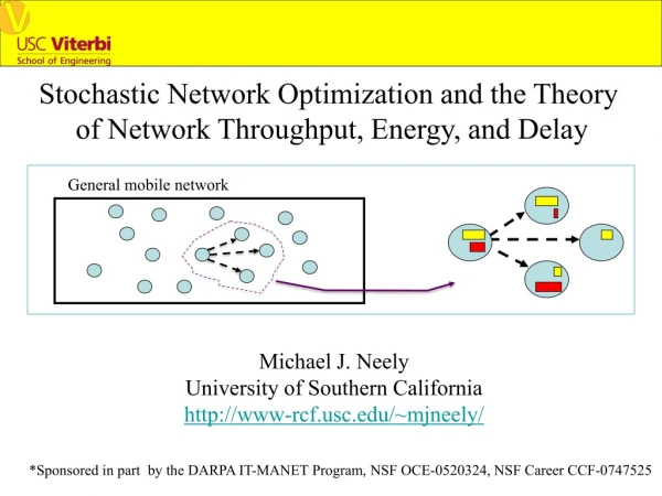
Delay Reduction via Lagrange Multipliers in Stochastic Network Optimization Longbo Huang Michael J. Neely EE@USC WiOpt 2009 *Sponsored in part by NSF Career CCF and DARPA IT-MANET Program
Outline • Problem formulation • Backlog behavior under Quadratic Lyapunov function based Algorithm (QLA): an example • General backlog behavior result of QLA for general SNO problems • The Fast-QLA algorithm (FQLA) • Simulation results • Summary
Problem Description: A Network of r Queues Slotted Time, t=0,1,2,… S(t) = Network State, Time-Varying, IID over slots (e.g. channel conditions, random arrivals, etc.) x(t) = Control Action, chosen in some abstract set X(S(t)) (e.g. power/bandwidth allocation, routing) (S(t), x(t)) costs: f(t)=f(S(t), x(t)) generates:Aj(t)=gj(S(t), x(t)) packets to queue j serves:μj(t)=bj(S(t), x(t)) packets in queue j [f(), g(), b() are only assumed to be non-negative, continuous, bounded] The stochastic problem: minimize: time average cost subject to: queue stability.
Problem Description: A Network of r Queues Slotted Time, t=0,1,2,… S(t) = Network State, Time-Varying, IID over slots (e.g. channel conditions, random arrivals, etc.) x(t) = Control Action, chosen in some abstract set X(S(t)) (e.g. power/bandwidth allocation, routing) (S(t), x(t)) costs: f(t)=f(S(t), x(t)) generates:Aj(t)=gj(S(t), x(t)) packets to queue j serves:μj(t)=bj(S(t), x(t)) packets in queue j [f(), g(), b() are only assumed to be non-negative, continuous, bounded] The stochastic problem: minimize: time average cost subject to: queue stability. QLA achieves: [G-N-T FnT 06] Avg. cost: fav <= f*av + O(1/V) Avg. Backlog: Uav <= O(V)
An Energy Minimization Example: The QLA algorithm μ1(t) μ2(t) μ3(t) μ4(t) μ5(t) R(t) U2 U3 U4 U1 U5 Goal: allocate power to support the flow with min avg. energy expenditure, i.e.: Min: avg. ΣiPi s.t. Queue stability S1(t) S2(t) S3(t) S4(t) S5(t) U2 W23(t) U3 Link 2->3 The QLA algorithm (built on Backpressure): 1. Compute the differentiable backlog Wii+1(t)=max[Ui(t)-Ui+1(t), 0], 2. Choose (P1(t), …P5(t) that maximizes: Σi[Wii+1(t)μi(Pi(t)) -VPi(t)] =Σi[Wii+1(t) Si(t) –V]Pi(t) e.g., if S2(t)=2, then if W23(t)*2>V, we set P2(t)=1.
An Energy Minimization Example: Backlog under QLA μ1(t) μ2(t) μ3(t) μ4(t) μ5(t) R(t) Goal: Min: avg. ΣiPi s.t. Queue stability U2 U3 U4 U1 U5 S1(t) S2(t) S3(t) S4(t) S5(t) Queue snapshot under QLA with V=100, first 100 slots: U1 U2 size U3 U4 U5 time
An Energy Minimization Example: Backlog under QLA μ1(t) μ2(t) μ3(t) μ4(t) μ5(t) R(t) Goal: Min: avg. ΣiPi s.t. Queue stability U2 U3 U4 U1 U5 S1(t) S2(t) S3(t) S4(t) S5(t) Queue snapshot under QLA with V=100, first 500 slots: U1 U2 size U3 U4 U5 time
An Energy Minimization Example: Backlog under QLA μ1(t) μ2(t) μ3(t) μ4(t) μ5(t) R(t) Goal: Min: avg. ΣiPi s.t. Queue stability U2 U3 U4 U1 U5 S1(t) S2(t) S3(t) S4(t) S5(t) Queue snapshot under QLA with V=100, first 1000 slots: U1 U2 size U3 U4 U5 time
An Energy Minimization Example: Backlog under QLA μ1(t) μ2(t) μ3(t) μ4(t) μ5(t) R(t) Goal: Min: avg. ΣiPi s.t. Queue stability U2 U3 U4 U1 U5 S1(t) S2(t) S3(t) S4(t) S5(t) Queue snapshot under QLA with V=100, first 5000 slots: U1 U2 size U3 U4 U5 time
An Energy Minimization Example: Backlog under QLA μ1(t) μ2(t) μ3(t) μ4(t) μ5(t) R(t) Goal: Min: avg. ΣiPi s.t. Queue stability U2 U3 U4 U1 U5 S1(t) S2(t) S3(t) S4(t) S5(t) Queue snapshot under QLA with V=100, (U1(t), U2(t)): (500,400) t=1:500k
An Energy Minimization Example: Backlog under QLA μ1(t) μ2(t) μ3(t) μ4(t) μ5(t) R(t) Goal: Min: avg. ΣiPi s.t. Queue stability U2 U3 U4 U1 U5 S1(t) S2(t) S3(t) S4(t) S5(t) Queue snapshot under QLA with V=100, (U1(t), U2(t)): (500,400) t=1:500k t=5k:500k
General result: Backlog under QLA Theorem 1: If q(U) satisfies C1: for some L>0 independent of V, then under QLA, in steady state, U(t) is mostly within O(log(V)) distance from UV* = Θ(V). Implications: (1) Delay under QLA is Θ(V), not just O(V); (2) The network stores a backlog vector ≈UV*.
General result: Backlog under QLA Theorem 1: If q(U) satisfies C1: for some L>0 independent of V, then under QLA, in steady state, U(t) is mostly within O(log(V)) distance from UV* = Θ(V). Implications: (1) Delay under QLA is Θ(V), not just O(V); (2) The network stores a backlog vector ≈UV*. Let’s “subtract out” UV* from the network! Replace most of the UV* data with Place-Holder bits
Fast-QLA (FQLA): Using place-holder bits A single queue example: First idea: (1) choose number of place-holder bits Q, s.t., if U(t0)>=Q, then U(t)>=Q for all t>=t0. (2) Let U(0)=Q, run QLA. Start here
Fast-QLA (FQLA): Using place-holder bits A single queue example: First idea: (1) choose number of place-holder bits Q, s.t., if U(t0)>=Q, then U(t)>=Q for all t>=t0. (2) Let U(0)=Q, run QLA. actual backlog Advantage: delay reduced by Q, same utility performance. Start here reduced
Fast-QLA (FQLA): Using place-holder bits A single queue example: First idea: (1) choose number of place-holder bits Q, s.t., if U(t0)>=Q, then U(t)>=Q for all t>=t0. (2) Let U(0)=Q, run QLA. actual backlog ≈Θ(V) Advantage: delay reduced by Q, same utility performance. Start here reduced Problem: Q ≈ UV*-Θ(V), delay Θ(V).
Fast-QLA (FQLA): Using place-holder bits A single queue example: FQLA idea: Choose # of place-holder bits Q such that backlog under QLA rarely goes below Q. Problem: (1) U(t) will eventually get below Q, what to do? (2) How to ensure utility performance?
Fast-QLA (FQLA): Using place-holder bits A single queue example: FQLA idea: Choose # of place-holder bits Q such that backlog under QLA rarely goes below Q. Problem: (1) U(t) will eventually get below Q, what to do? (2) How to ensure utility performance? Answer: use virtual backlog process W(t) + careful pkt dropping
Fast-QLA (FQLA): Using place-holder bits A single queue example: FQLA: (1) Choose # of place-holder bits Q such that backlog under QLA rarely goes below Q. (2) Use a virtual backlog process W(t) with W(0)=Q to track the backlog that should have been generated by QLA. (3) Obtain action by running QLA based on W(t), modify the action carefully.
Fast-QLA (FQLA): Using place-holder bits A single queue example: If W(t)>=Q, same as QLA, admit A(t), serve μ(t), i.e., FQLA=QLA. If W(t)<Q, serve μ(t), only admit: A’(t)=max[A(t)-(Q-W(t)), 0]. This modification ensures: U(t) ≈ max[W(t)-Q, 0]. Modifying the action
Fast-QLA (FQLA): Using place-holder bits A single queue example: If W(t)>=Q, same as QLA, admit A(t), serve μ(t), i.e., FQLA=QLA. If W(t)<Q, serve μ(t), only admit: A’(t)=max[A(t)-(Q-W(t)), 0]. This modification ensures: U(t) ≈ max[W(t)-Q, 0]. Modifying the action
Fast-QLA (FQLA): Using place-holder bits A single queue example: If W(t)>=Q, same as QLA, admit A(t), serve μ(t), i.e., FQLA=QLA. If W(t)<Q, serve μ(t), only admit: A’(t)=max[A(t)-(Q-W(t)), 0]. This modification ensures: U(t) ≈ max[W(t)-Q, 0]. Modifying the action
Fast-QLA (FQLA): Using place-holder bits A single queue example: If W(t)>=Q, same as QLA, admit A(t), serve μ(t), i.e., FQLA=QLA. If W(t)<Q, serve μ(t), only admit: A’(t)=max[A(t)-(Q-W(t)), 0]. This modification ensures: U(t) ≈ max[W(t)-Q, 0]. Modifying the action
Fast-QLA (FQLA): Using place-holder bits A single queue example: If W(t)>=Q, same as QLA, admit A(t), serve μ(t), i.e., FQLA=QLA. If W(t)<Q, serve μ(t), only admit: A’(t)=max[A(t)-(Q-W(t)), 0]. This modification ensures: U(t) ≈ max[W(t)-Q, 0]. Modifying the action
Fast-QLA (FQLA): Using place-holder bits A single queue example: If W(t)>=Q, same as QLA, admit A(t), serve μ(t), i.e., FQLA=QLA. If W(t)<Q, serve μ(t), only admit: A’(t)=max[A(t)-(Q-W(t)), 0]. This modification ensures: U(t) ≈ max[W(t)-Q, 0]. Modifying the action
Fast-QLA (FQLA): Using place-holder bits A single queue example: If W(t)>=Q, same as QLA, admit A(t), serve μ(t), i.e., FQLA=QLA. If W(t)<Q, serve μ(t), only admit: A’(t)=max[A(t)-(Q-W(t)), 0]. This modification ensures: U(t) ≈ max[W(t)-Q, 0]. Now choose: Q=max[UV*-log2(V), 0] (1) ensures: Low delay: average U ≈ log2(V), (2) ensures W(t) rarely below Q, implying: Good utility & few pkt dropped: very few action modifications. Modifying the action
Fast-QLA (FQLA): Performance Theorem 2: If condition C1 in Theorem 1 holds, then we have under FQLA-Ideal: Recall: under QLA:
Simulation R(t) • Simulation parameters: • V= 50, 100, 200, 500, 1000, 2000, • Each with 5x10⁶ slots, • UV*=(5V, 4V, 3V, 2V, V)T. U2 U3 U4 U1 U5 S1(t) S2(t) S3(t) S4(t) S5(t) Backlog % of pkt dropped
Simulation R(t) • Simulation parameters: • V= 50, 100, 200, 500, 1000, 2000, • Each with 5x10⁶ slots, • UV*=(5V, 4V, 3V, 2V, V)T. U2 U3 U4 U1 U5 S1(t) S2(t) S3(t) S4(t) S5(t) Sample (W1(t),W2(t)) process: V=1000, t=10000:110000 Note: W1(t)>Q1=4952 & W2(t)>Q2=3952
Simulation R(t) • Simulation parameters: • V= 50, 100, 200, 500, 1000, 2000, • Each with 5x10⁶ slots, • UV*=(5V, 4V, 3V, 2V, V)T. U2 U3 U4 U1 U5 S1(t) S2(t) S3(t) S4(t) S5(t) Quick comparison V=1000, U QLA≈15V=15000 U FQLA≈5log2(V)=250 60times better! Backlog % of pkt dropped
Summary • Under QLA, the backlog vector usually stays close to an “attractor” – the optimal Lagrange multiplier UV*. • FQLA subtracts out the Lagrange multiplier from the system induced by QLA by using place-holder bits to reduce delay.
Summary • Under QLA, the backlog vector usually stays close to an “attractor” – the optimal Lagrange multiplier UV*. • FQLA subtracts out the Lagrange multiplier from the system induced by QLA by using place-holder bits to reduce delay. Note: (1) Theorem 1 also holds when S(t) is Markovian, (2) FQLA-General for the case where UV* is not known, performance similar to FQLA-Ideal, (3) when q0(U) is “smooth”, we prove O(sqrt{V}) deviation bound, (4) The “Network Gravity” role of Lagrange multiplier. Details see ArXiv report 0904.3795
Thank you ! Questions or Comments?