U N I T .

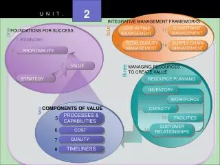
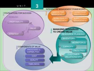
1. FOUNDATIONS FOR SUCCESS one Introduction PROFITABILITY VALUE STRATEGY WORKFORCE CAPACITY INVENTORY FACILITIES SUPPLY CHAIN MANAGEMENT JUST-IN-TIME MANAGEMENT CONSTRAINT MANAGEMENT TOTAL QUALITY MANAGEMENT 3 U N I T . INTEGRATIVE MANAGEMENT FRAMEWORKS 17 four 15 1 16 18 2 3 MANAGING RESOURCES TO CREATE VALUE three 4 RESOURCE PLANNING 9 10 11 12 COMPONENTS OF VALUE two PROCESSES & CAPABILITIES 13 5 CUSTOMER RELATIONSHIPS 14 COST 6 QUALITY 7 TIMELINESS 8

2. L E A R N I N G O B J E C T I V E S 10 C H A P T E R Inventory • Explain why businesses carry inventory. • Describe the costs associated with inventory. • Compare independent and dependent demand inventory. • Calculate days-of-supply. • Explain how a reorder point system works. • Describe the contribution made by a safety stock. • Compute the reorder point for a desired service level. • Describe weaknesses of the economic order quantity. • Compute the appropriate order quantity for a fixed interval variable quantity system. • Describe the information inputs necessary to manage dependent demand inventory. • Compute planned order releases using material requirements planning. • Explain ABC analysis.

3. A Balancing Act for Management • The first of five resource categories. Exhibit 10.1 The Role of Inventory in the Resource/ Profit Model

4. Why Carry Inventory? • Decoupling: reducing direct dependencies. • Disruptions, if decoupled, don’t have as serious of an impact. • Decoupling enhances reliability and response time.

5. Why Avoid Too Much Inventory? • The investment doesn’t provide a financial return. • Costs of storage, insurance, and other costs are high.

6. Types of Inventory: Costs and Benefits • Inventories decouple customer from supplier, one machine for another, and provide flexibility. • Order costs: the administrative cost associated with ordering. • Carrying costs: costs linked to the level of inventory. • Setup or changeover: analogous to ordering cost, but costs incurred for manufacturers. • Stockout costs: costs associated with running out or not having inventory. • Purchasing cost: usually independent of inventory level

7. Carrying Costs Are Linked to the Average Level of Inventory Exhibit 10.2 Average Inventory as Q/2

8. Example 10.1: Days-of-Supply Calculation • Calculate days of supply when average demand is 40 gallons per day, and 60 gallons remain. • Solution: On hand inventory = 1.5 Average demand Excel Tutor 10.1

9. Delivery Patterns • Frequent deliveries of small quantities result in lower average levels of inventory than infrequent deliveries of large quantities. Exhibit 10.3 Frequent Small Deliveries versus Infrequent Large Deliveries

10. Retailing and Finished Product Inventories • Days of supply is often used to describe how much is available. Exhibit 10.4 Example of Day’s Supply

11. Inventory as a Buffer of Demand Variability • Manufacturers use inventory to help level production when demand is variable. • Storing inventory during low-demand times and using it when demand is higher than production rate. Exhibit 10.5 Inventory to Buffer Against Seasonal Demand

12. Independent Demand Inventory • Retail, finished product inventories of manufacturers, and MRO inventories are called independent demand inventories. • The demand is dictated by a market. • The only way to know what the demand will be in advance is to forecast it.

13. Dependent Demand Inventories • Component parts, raw materials, and work-in-process inventory of manufacturers is known as dependent demand inventory. • Dependent demand inventory is dictated by a production schedule. • Dependent demand can be calculated precisely, it need not be forecast.

14. Inventory Decisions • Two critical questions for managing inventory: • When should inventory be ordered? • How much should be ordered?

15. Managing Independent Demand Inventory • Independent demand is uncertain. • The percent of demand met is the service level. • The amount of time you must wait for an order is the replenishment lead time. • Since there is a replenishment lead time, orders must be made before the inventory has run out. • Two general approaches: • Fixed quantity, variable interval systems • Fixed interval, variable quantity systems

16. Fixed Quantity, Variable Interval System: The Reorder Point Model • Inventory is reordered when there is enough inventory remaining to meet demand during the replenishment lead time. • Demand during the replenishment lead time is uncertain. Exhibit 10.6 Distribution of Demand During Lead Time

17. Fixed Quantity, Variable Interval System: The Reorder Point Model • To meet demand during the replenishment lead time, the reorder point must include a safety stock linked to demand variability. • Reorder point = _ dLT + sLTZ

18. Fixed Quantity, Variable Interval System: The Reorder Point Model Exhibit 10.7 Reorder Point System

19. Fixed Quantity, Variable Interval System: The Reorder Point Model Exhibit 10.8 ROP at 2.33s Interactive Model 10.1

20. Example 10.2: Reorder Point Calculation • Lead time is 2 weeks, average weekly demand is 62. • Weekly standard deviation is 13. • Compute a reorder point with a 95% service level. • Solution: Average demand during lead time = 124 Standard deviation of demand during the lead time = 18.38 Z for a 95% service level – 1.645 (from appendix A) _ ROP = dLT + Sltz ROP = 154.243 Excel Tutor 10.2

21. How Many to Order: Economic Order Quantity • Total Cost = H(Q/2) + S(D/Q) • H = carrying cost per unit, annually • Q = order quantity • S = order cost • D = annual demand • EOQ = 2DS H

22. How Many to Order: Economic Order Quantity Exhibit 10.9 Holding Costs, Order Costs, and Total Costs in EOQ

23. Example 10.3: Economic Order Quantity Calculation • D = 600 per year, S = $13 per order, H = 3.25 per year. EOQ = 2 (600)(13) 3.25 = 69.28203 Interactive Model 10.2 Excel Tutor 10.3

24. Quantity Discounts • If quantity discounts are offered, the total cost must include the actual cost of the items ordered, since it varies along with order cost and carrying cost. • The computation process is to first compute the EOQ and the total cost at the EOQ. The total cost of all lower priced price ranges must be computed and compared.

25. Example 10.4 Quantity Discount Model Calculation • Given the following information, compute the low-cost order quantity. 1-20 units: $229 each; 21-60 units: 210 each; 61-120 units: $199 each; and over 120 units: $165 each. Order cost: $20 per order; Carrying cost =$36 per unit per year; Annual demand: 476 • Solution:Basic EOQ = 22.997, TC at EOQ = $100,787.91 TC of ordering 61 units = $95,978.07 TC or ordering 121 units = $85,556.68 Order 121 units. Excel Tutor 10.4

26. Fixed Interval Variable Quantity Systems • Known as a “periodic review” system. • Order is placed on fixed intervals, and the quantity varies. • Fixed interval systems are exposed to stockout at any time, whereas reorder point systems are only at risk during the replenishment lead time. • Order quantity = expected demand during the order interval and replenishment lead time • Plus, a safety stock • Minus, any inventory on hand at the time the order is placed.

27. Fixed Interval Variable Quantity Systems Exhibit 10.10 Periodic Review System

28. Example 10.5: Periodic Review Model Calculation • Average daily demand: 3.6 units; lead time: 2 days; standard deviation of demand over the order interval an lead time: 1.4; Inventory currently on hand: 5 units; Service level 99%, order interval: 7 days. • Solution: • Q = dOI+LT + sdZ (OI + LT) – A = 32.4 + 4.786 = 37.186 Excel Tutor 10.5

29. Managing Dependent Demand Inventory • Demand is calculated using Material Requirements Planning (MRP) logic • MRP seeks to answer the same 2 questions: • When to order • How much to order. • When? Requires computing when to order, given that we know when it is due. This is a “backward scheduling” process. • How much? Requires calculating what is needed, given that some inventory already exists. This is known as “netting.”

30. Managing Dependent Demand Inventory • Inputs to MRP logic: • Master Production Schedule (MPS) provides the production schedule for the end items. • Bill of Material provides the product structure so we know which components are needed for the end item. • Inventory master file tells us how many are currently on hand, and information such as order policies, sources, etc.

31. Managing Dependent Demand Inventory Exhibit 10.11 Material Requirements Planning Inputs

32. Managing Dependent Demand Inventory Exhibit 10.13 Structure for Staple Remover

33. Managing Dependent Demand Inventory

34. Managing Dependent Demand Inventory

35. Managing Dependent Demand Inventory Exhibit 10.15 continued

36. Managing Dependent Demand Inventory Exhibit 10.16 Time Line for Staple Remover

37. ABC Analysis for Prioritizing Inventory • System management can be expensive. • System sophistication (cost) should be relative to the cost of stocking out. • A items are most critical and warrant the most expensive system. • B items are less critical and would need a less expensive system. • C items are relatively unimportant. Reel Operations 10.1

38. Inventory Productivity • Inventory Turns: sales/average value of inventory • Dollar Days: value of inventory x the number of days until sold

39. Example 10.7: Dollar-Day Calculation • Camcorder value: $1000; annual demand = 730; 12 units on hand • 35mm camera value: $214.29; annual demand = 52 units; 7 units on hand.

40. Example 10.7: Dollar-Day Calculation Excel Tutor 10.7