Download
1 / 9
100 likes | 248 Vues
Explore complex root solutions in differential equations, including Euler's formula and obtaining real-valued solutions. Learn how to find a fundamental solution set and express the general solution. Work through examples to understand applying these concepts and solve initial value problems.

E N D
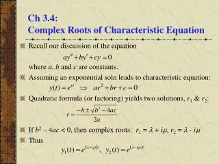
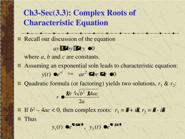
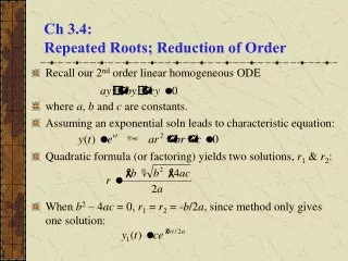
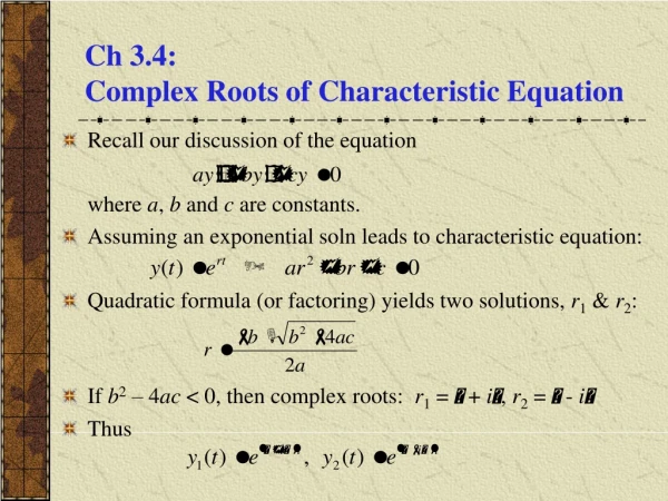
Ch 3.4: Complex Roots of Characteristic Equation • Recall our discussion of the equation where a, b and c are constants. • Assuming an exponential soln leads to characteristic equation: • Quadratic formula (or factoring) yields two solutions, r1 & r2: • If b2 – 4ac < 0, then complex roots: r1 = + i, r2 = - i • Thus
Euler’s Formula; Complex Valued Solutions • Substituting it into Taylor series for et, we obtain Euler’s formula: • Generalizing Euler’s formula, we obtain • Then • Therefore
Real Valued Solutions • Our two solutions thus far are complex-valued functions: • We would prefer to have real-valued solutions, since our differential equation has real coefficients. • To achieve this, recall that linear combinations of solutions are themselves solutions: • Ignoring constants, we obtain the two solutions
Real Valued Solutions: The Wronskian • Thus we have the following real-valued functions: • Checking the Wronskian, we obtain • Thus y3 and y4 form a fundamental solution set for our ODE, and the general solution can be expressed as
Example 1 • Consider the equation • Then • Therefore and thus the general solution is
Example 2 • Consider the equation • Then • Therefore and thus the general solution is
Example 3 • Consider the equation • Then • Therefore the general solution is
Example 4: Part (a) (1 of 2) • For the initial value problem below, find (a) the solution u(t) and (b) the smallest time T for which |u(t)| 0.1 • We know from Example 1 that the general solution is • Using the initial conditions, we obtain • Thus
Example 4: Part (b) (2 of 2) • Find the smallest time T for which |u(t)| 0.1 • Our solution is • With the help of graphing calculator or computer algebra system, we find that T 2.79. See graph below.