Download
1 / 49
490 likes | 614 Vues
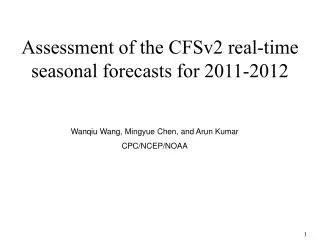
How Does NCEP/CPC Make Operational Monthly and Seasonal Forecasts?. Huug van den Dool (CPC) CPC, June 23, 2011/ Oct 2011/ Feb 15, 2012 / UoMDMay,2,2012/ Aug2012/ Dec,12,2012/UoMDApril24,2013/ May22,2013/. Assorted Underlying Issues. Which tools are used… How do these tools work?

E N D
How Does NCEP/CPC Make Operational Monthly and Seasonal Forecasts? Huug van den Dool (CPC) CPC, June 23, 2011/ Oct 2011/ Feb 15, 2012 / UoMDMay,2,2012/ Aug2012/ Dec,12,2012/UoMDApril24,2013/ May22,2013/
Assorted Underlying Issues • Which tools are used… • How do these tools work? • How are tools combined??? • Dynamical vs Empirical Tools • Skill of tools and OFFICIAL • How easily can a new tool be included? • US, yes, but occasional global perspective • Physical attributions
Menu of CPC predictions: 6-10 day (daily) Week 2 (daily) Monthly (monthly + update) Seasonal (monthly) Other (hazards, drought monitor, drought outlook, MJO, UV-index, degree days, POE, SST) (some are ‘briefings’) Informal forecast tools (too many to list) http://www.cpc.ncep.noaa.gov/products/predictions/90day/tools/briefing/index.pri.html
EXAMPLE P U B L I C L Y I S S U E D “ O F F I C I A L ” F O R E C A S T
EMP EMP EMP EMP N/A DYN CON CON EMP DYN
SMLR CCA OCN LAN OLD-OTLK CFSV1 LFQ ECP IRI ECA CON 9 (15 CASES: 1950, 54, 55, 56, 64, 68, 71, 74, 75, 76, 85, 89, 99, 00, 08)
Element US-T US-P SST US-soil moisture Method:CCA X X X OCN X X CFS X X X XSMLR X XECCA X XConsolidation X X X Constr Analog X X X XMarkov X ENSO Composite X X Other (GCM) models (IRI, ECHAM, NCAR, N(I)MME): X X CCA = Canonical Correlation AnalysisOCN = Optimal Climate NormalsCFS = Climate Forecast System (Coupled Ocean-Atmosphere Model)SMLR = Stepwise Multiple Linear RegressionCON = Consolidation
About OCN. Two contrasting views:- Climate = average weather in the past- Climate is the ‘expectation’ of the future30 year WMO normals: 1961-1990; 1971-2000; 1981-2010 etcOCN = Optimal Climate Normals: Last K year average. All seasons/locations pooled: K=10 is optimal (for US T).Forecast for Jan 2012 (K=10) = (Jan02+Jan03+... Jan11)/10. – WMO-normalplus a skill evaluation for some 50+ years.Why does OCN work?1) climate is not constant (K would be infinity for constant climate)2) recent averages are better3) somewhat shorter averages are better (for T)see Huang et al 1996. J.Climate. 9, 809-817.
OCN has become the bearer of most of the skill, see also EOCN method (Peng et al)
G H C N - C A M S F A N 2 0 0 8
NCEP’s Climate Forecast System, now called CFS v2 • MRFb9x, CMP12/14, 1995 onward (Leetmaa, Ji etc). Tropical Pacific only. • SFM 2000 onward (Kanamitsu et al • CFSv1, Aug 2004, Saha et al 2006. Almost global ocean • CFSR, Saha et al 2010 • CFSv2, March 2011. Global ocean, interactive sea-ice, increases in CO2.
Major Verification Issues ‘a-priori’ verification (used to be rare) After the fact (fairly normal)
After the fact….. Source Peitao Peng
(Seasonal) Forecasts are useless unless accompanied by a reliable a-priori skill estimate.Solution: develop a 50+ year track record for each tool. 1950-present.(Admittedly we need 5000 years)
OFFicial Forecast(element, lead, location, initial month) = a * A + b * B + c * C +…Honest hindcast required 1950-present. Covariance (A,B), (A,C), (B,C), and(A, obs), (B, obs), (C, obs) allows solution for a, b, c (element, lead, location, initial month)
Fig.7.6: The skill (ACX100) of forecasting NINO34 SST by the CA method for the period 1956-2005. The plot has the target season in the horizontal and the lead in the vertical. Example: NINO34 in rolling seasons 2 and 3 (JFM and FMA) are predicted slightly better than 0.7 at lead 8 months. An 8 month lead JFM forecast is made at the end of April of the previous year. A 1-2-1 smoothing was applied in the vertical to reduce noise. CA skill 1956-2005
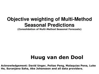
M. Peña Mendez and H. van den Dool, 2008: Consolidation of Multi-Method Forecasts at CPC. J. Climate, 21, 6521–6538. Unger, D., H. van den Dool, E. O’Lenic and D. Collins, 2009: Ensemble Regression. Monthly Weather Review, 137, 2365-2379. (1) CTB, (2) why do we need ‘consolidation’?
SEC SEC and CV 3CVRE
See also: O’Lenic, E.A., D.A. Unger, M.S. Halpert, and K.S. Pelman, 2008: Developments in Operational Long-Range Prediction at CPC.Wea. Forecasting, 23, 496–515.
Empirical tools can be comprehensive! (Thanks to reanalysis, among other things). And very economic.Constructed Analogue(next 2 slides)
Given an Initial Condition, SSTIC (s, t0) at time t0 . We express SSTIC (s, t0) as a linear combination of all fields in the historical library, i.e. 2010 • SSTIC (s, t0) ~= SSTCA(s) = Σ α(t) SST(s,t) (1) t=1956 (CA=constructed Analogue) • The determination of the weights α(t) is non-trivial, but except for some pathological cases, a set of (55) weights α(t) can always be found so as to satisfy the left hand side of (1), for any SSTIC , to within a tolerance ε.
Equation (1) is purely diagnostic. We now submit that given the initial condition we can make a forecast with some skill by 2010 • XF (s, t0+Δt) = Σ α(t) X(s, t +Δt) (2) t=1956 Where X is any variable (soil moisture, temperature, precipitation) • The calculation for (2) is trivial, the underlying assumptions are not. We ‘persist’ the weights α(t) resulting from (1) and linearly combine the X(s,t+Δt) so as to arrive at a forecast to which XIC (s, t0) will evolve over Δt.
Z500 SST CA T2m Precip
SST Z500 CFS T2m Precip Source: Wanqiu Wang
Physical attributions of Forecast Skill • Global SST, mainly ENSO. Tele-connections needed. • Trends, mainly (??) global change • Distribution of soil moisture anomalies
Website for display of NMME&IMMENMME=National Multi-Model EnsembleIMME=International Multi-Model Ensemble • http://origin.cpc.ncep.noaa.gov/products/NMME/
Please attend • Friday 2pm June 14 • Tuesday 1:30pm June 18 Two meetings to Discuss the Seasonal Forecast.