Advanced Wave Equation Migration Techniques for Enhanced Seismic Imaging at SEG 2005
250 likes | 387 Vues
This presentation outlines innovative wave equation migration tools developed as part of a long-term R&D effort. Covering both 2D and 3D methodologies—including paraxial propagators and common-offset wavefield migration—the focus is on achieving true amplitude wavefield migration. The software supports various one-way propagation methods, optimizing accuracy in complex velocity scenarios. Designed for scalability, it employs multifaceted parallelization strategies to handle large datasets efficiently, making it crucial for modern seismic analysis and imaging applications.

Advanced Wave Equation Migration Techniques for Enhanced Seismic Imaging at SEG 2005
E N D
Presentation Transcript
Presentation of the Wave Equation Migration tool 75th SEG Annual Meeting, Houston, TX. November 6 - 11, 2005.
Long term R&D effort • 2D Paraxial propagator (Collino, 1989) • Constrained least squares migration (Ehinger and Lailly, 1991; Duquet et al., 1994) • Common offset wavefield migration (Ehinger et al.; 1996) • 3D paraxial propagator (Collino and Joly, 1995) • 3D prestack wavefield migration (Duquet et al., 2001) • Comparison of 3D wavefield propagator (Lavaud and Duquet, 2001) • True amplitude wavefield migration (Joncour et al., 2005)
WE Method • Shot record Migration • Accurate • No assumption on the propagation complexity • No assumption on the acquisition geometry • Easy parallelization (shot, frequencies, ...) • Various One-Way propagation kernel • Finite Difference methods, Wavenumber methods, Mixed methods
One-Way propagation methods • Two main approaches : Finite Difference and Wavenumber • Finite difference (paraxial) : • Handle strong lateral velocity variations • Dip limited • Anisotropic Error in 3D (splitting method) • Wanenumber (SSF, PSPI) : • Handle gentle velocity variations • High dip accurate • Isotropic Error • Mixed method (FFD, Li) : • Combine both approaches
Accuracy of FD propagation 2 splitting directions 4 splitting directions 45 ° 68 °
One-Way propagation method • All these methods are implemented in our software namely: • SSF, PSPI, FD, FFD, LI, Optimized Li • FD propagation kernel: • 2 or 4 splitting directions • Unconditionally stable
Synthetic model Strong velocity contrasts + High dips Layer 1 = homogeneous velocity 1.5 km/s Layer 2 = layer 4 = lateral velocity gradient from 2 to 3 km/s Layer 3 = vertical velocity gradient from 3 to 4 km/s Layer 5 = homogeneous velocity 4 km/s
WE software • 2D/3D shot record migration • Common Angle Gather • Different parallelization level • Optimization strategy • Designed for huge size problem
Master Node Shot parallelization Slave Node n Slave Node 1 Frequency parallelization proc 1 proc 1 proc n proc n Two level parallelization
Two level parallelization • Coarse grain parallelization over shots • Masternode assign and send shared shots to each Slave node • Finer grain parallelization over frequency • Slavenode can be a dual/quadri processor or a cluster subset • mpi parallelization: each processor takes a subset of the frequencies • Reduced communication: • data reading + image condition
Optimization strategy • Shared shot allow to save cost associated with propagation matrix construction • Large step through water • Propagation depth step can be bigger than imaging depth step using an ad'hoc interpolation • ...
dz image=40m / dz propagation=40m 4 times faster
dz image=10m / dz propagation=40m+ ad'hoc interpolation 3 times faster
Designed for huge size problem • Memory requirement • Lateral propagation domain : 15km x 10km • Spatial sampling dx=dy=25m • Recording time= 10s • Frequency band = 40Hz (400 frequencies) • ~2 Gb core memory • Flexibility on the frequency range to be migrated
WE software • Shot record migration • accurate method • Fast and flexible algorithm • Various propagation kernels • handle high dips and strong velocity contrasts